SCGraph
August 31, 2026 · View on GitHub



A high-performance, lightweight Python library for shortest path routing on geographic and supply chain networks.
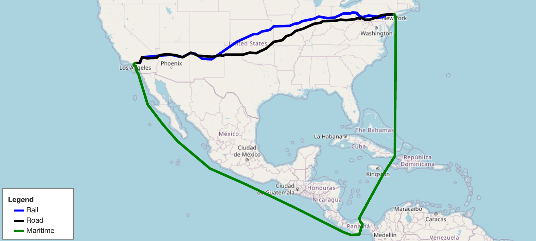
SCGraph provides fast, flexible shortest path routing for road, rail, maritime, and custom networks. It ships with prebuilt geographic networks, supports arbitrary graph construction and OSMNx integration, and scales from simple point-to-point queries to massive distance matrices. It also supports graph reduction, lazy loading, optional C++ acceleration, and Contraction Hierarchy preprocessing for large-scale applications.
- Docs: https://connor-makowski.github.io/scgraph/scgraph.html
- Paper: https://ssrn.com/abstract=5388845
- Award: 2025 MIT Prize for Open Data
Citation
If you use SCGraph in your research, please cite:
Makowski, C., Saragih, A., Guter, W., Russell, T., Heinold, A., & Lekkakos, S. (2025). SCGraph: A Dependency-Free Python Package for Road, Rail, and Maritime Shortest Path Routing Generation and Distance Estimation. MIT Center for Transportation & Logistics Research Paper Series, (2025-028). https://ssrn.com/abstract=5388845
@article{makowski2025scgraph,
  title={SCGraph: A Dependency-Free Python Package for Road, Rail, and Maritime Shortest Path Routing Generation and Distance Estimation},
  author={Makowski, Connor and Saragih, Austin and Guter, Willem and Russell, Tim and Heinold, Arne and Lekkakos, Spyridon},
  journal={MIT Center for Transportation & Logistics Research Paper Series},
  number={2025-028},
  year={2025},
  url={https://ssrn.com/abstract=5388845}
}
Installation
pip install scgraph
A C++ extension is compiled automatically if a C++ compiler is available (~10x speedup on core algorithms). To verify: from scgraph.utils import cpp_check; cpp_check().
To skip the C++ build:
# macOS / Linux / WSL2
export SKBUILD_CMAKE_ARGS="-DSKIP_CPP_BUILD=ON" && pip install scgraph
# Windows (PowerShell)
$env:SKBUILD_CMAKE_ARGS="-DSKIP_CPP_BUILD=ON"; pip install scgraph
# Windows (CMD)
set SKBUILD_CMAKE_ARGS=-DSKIP_CPP_BUILD=ON && pip install scgraph
Quick Start: Using Built-in GeoGraphs
Get the shortest maritime path between Shanghai and Savannah, GA:
from scgraph import GeoGraph

marnet_geograph = GeoGraph.load_geograph("marnet")

output = marnet_geograph.get_shortest_path(
    origin_node={"latitude": 31.23, "longitude": 121.47},
    destination_node={"latitude": 32.08, "longitude": -81.09},
    output_units='km',
)
print(output['length'])  #=> 19596.4653
The output dictionary always contains:
| Key | Description |
|---|---|
length | Distance along the shortest path in the requested output_units |
coordinate_path | List of [latitude, longitude] pairs making up the path |
Built-in Geographs
All built-in geographs measure distances in kilometers and are downloaded on first use and cached locally.
| Name | Load Key | Description | Attribution |
|---|---|---|---|
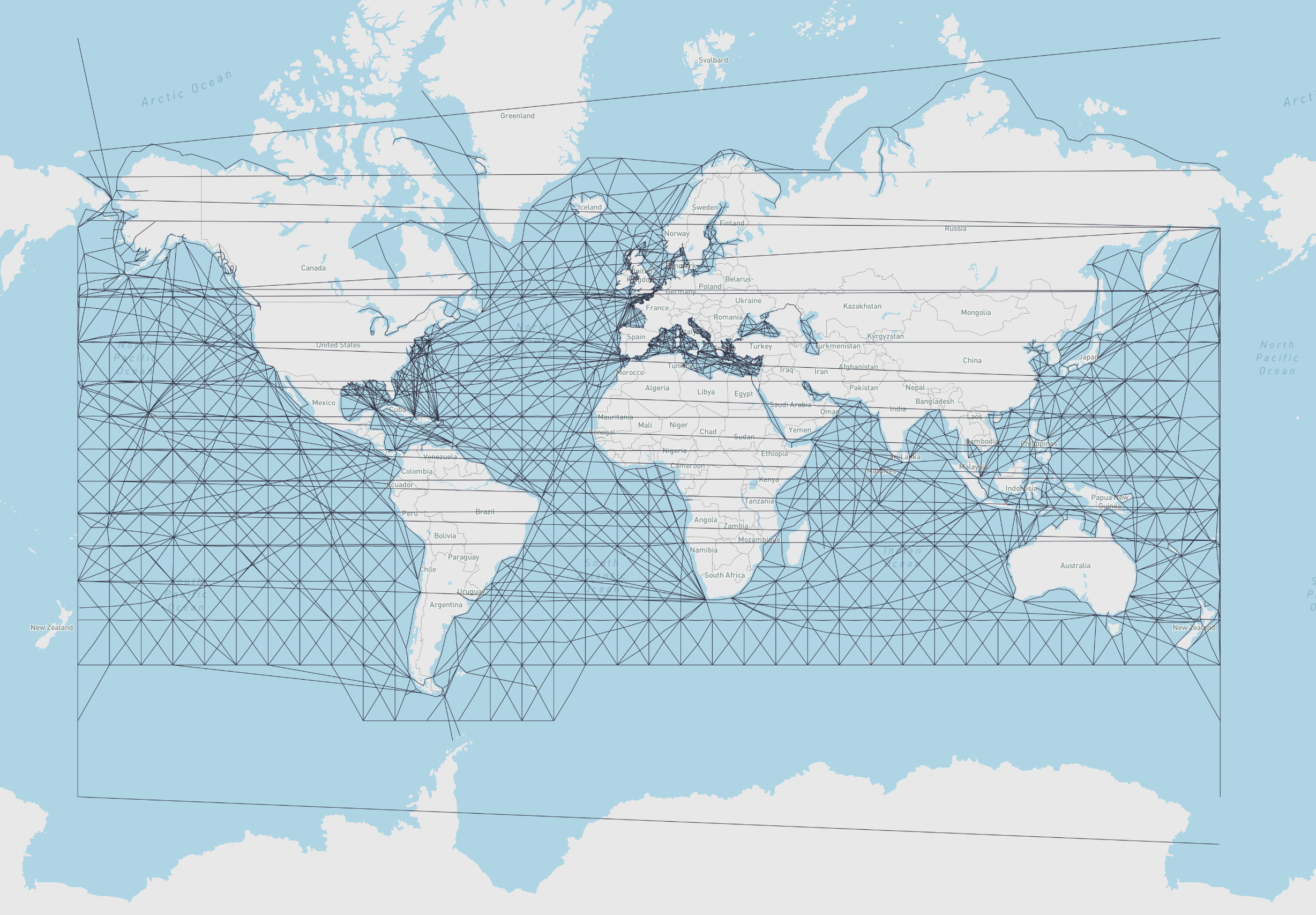
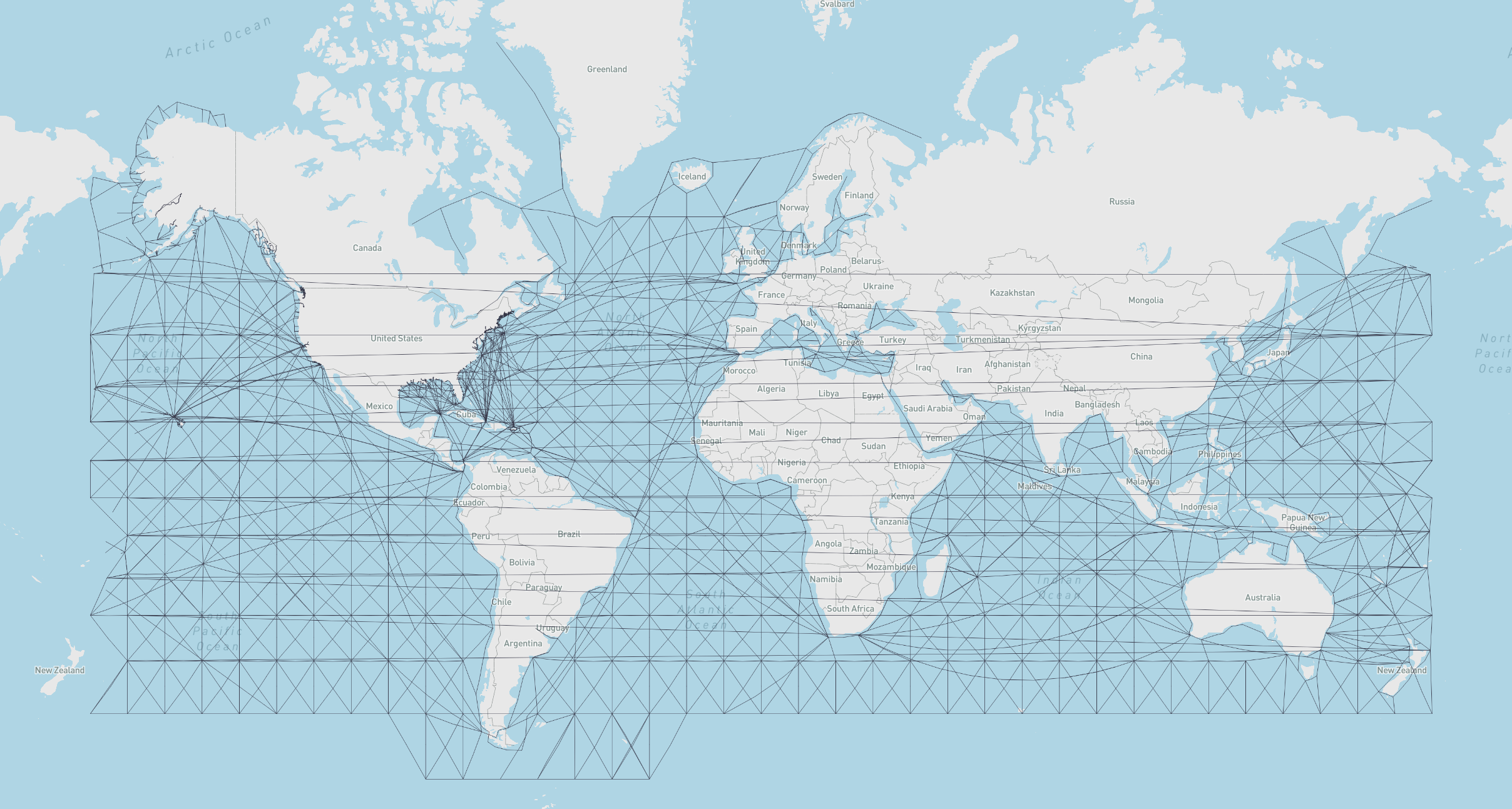
marnet | GeoGraph.load_geograph("marnet") | Maritime network | searoute · Map |
oak_ridge_maritime | GeoGraph.load_geograph("oak_ridge_maritime") | Maritime network (Oak Ridge National Laboratory) | ORNL / Geocommons · Map |
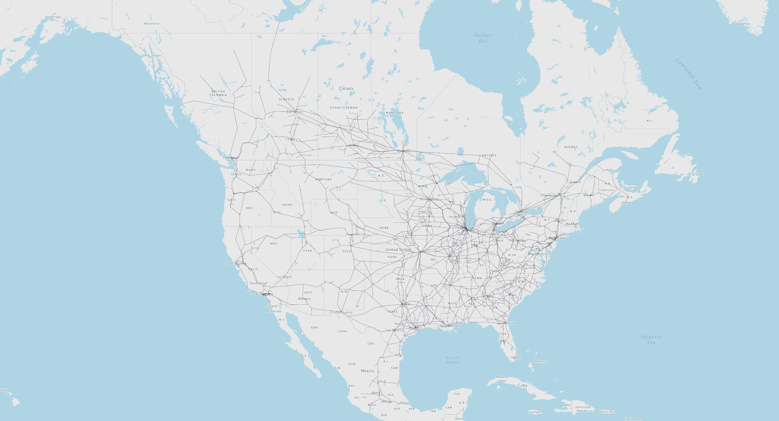
north_america_rail | GeoGraph.load_geograph("north_america_rail") | Class 1 rail network for North America | USDOT ArcGIS · Map |
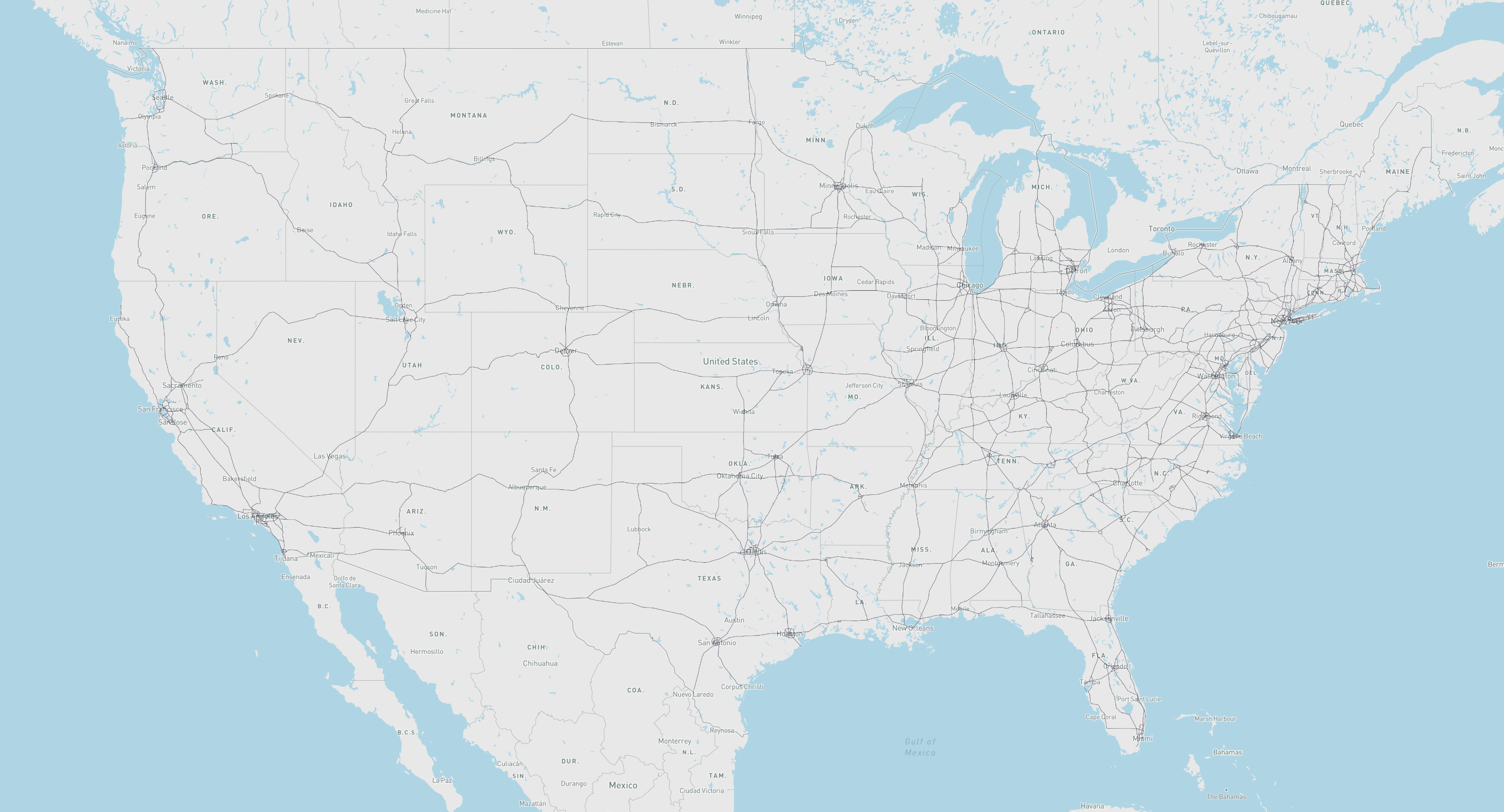
us_freeway | GeoGraph.load_geograph("us_freeway") | Freeway network for the United States | USDOT ArcGIS · Map |
world_highways_and_marnet | GeoGraph.load_geograph("world_highways_and_marnet") | World highway network merged with the maritime network | OpenStreetMap / searoute |
world_highways | GeoGraph.load_geograph("world_highways") | World highway network | OpenStreetMap |
world_railways | GeoGraph.load_geograph("world_railways") | World railway network | OpenStreetMap |
Quick Start: OSMNx Integration
Route on any OpenStreetMap network (including bike, drive, and walk) using OSMNx. This example finds the fastest and shortest bike paths between two points in Somerville and Cambridge, MA, then cross-evaluates each path's time and distance:
import osmnx as ox
from scgraph import GeoGraph

# Download the bike network for Somerville and Cambridge, MA
G = ox.graph_from_place(
    ['Somerville, Massachusetts, USA', 'Cambridge, Massachusetts, USA'],
    network_type='bike'
)
G = ox.add_edge_speeds(G)
G = ox.add_edge_travel_times(G)

# Build a time-based and a distance-based GeoGraph from the same OSMNx graph
geograph_time     = GeoGraph.load_from_osmnx_graph(G, weight_key='travel_time')
geograph_distance = GeoGraph.load_from_osmnx_graph(G, weight_key='length')

origin      = {'latitude': 42.3601, 'longitude': -71.0942}  # MIT campus
destination = {'latitude': 42.3876, 'longitude': -71.0995}  # Somerville City Hall

time_result     = geograph_time.get_shortest_path(origin_node=origin, destination_node=destination, output_path=True)
distance_result = geograph_distance.get_shortest_path(origin_node=origin, destination_node=destination, output_path=True)

# Cross-evaluate: get the distance of the time-optimal path, and vice versa
time_path_distance_km = geograph_distance.get_path_weight(time_result)
distance_path_time_s  = geograph_time.get_path_weight(distance_result)

print(f"Time-optimal path:     {time_result['length']:.1f} s  |  {time_path_distance_km:.3f} km")
print(f"Distance-optimal path: {distance_path_time_s:.1f} s  |  {distance_result['length']:.3f} km")
# Time-optimal path:     340.9 s  |  3.920 km
# Distance-optimal path: 369.3 s  |  3.605 km
See the OSMNx notebook for a full example with folium map visualization.
Core Concepts
What is a GeoGraph?
A GeoGraph is the primary object in SCGraph. It combines a graph (a network of nodes and weighted edges) with geographic coordinates (latitude/longitude for each node), enabling shortest path queries between arbitrary real-world coordinates, not just predefined graph nodes.
When you call get_shortest_path, SCGraph:
- Temporarily inserts your origin and destination as new nodes in the graph
- Connects them to nearby graph nodes using haversine or euclidean distance
- Runs the requested shortest path algorithm
- Returns the path in geographic coordinates
- Cleans up the temporary nodes
This means you never need to worry about whether your start/end points are "in" the network. SCGraph handles that automatically.
Graph Structure
Internally, a graph is represented as a list of adjacency dicts:
graph = [
    {1: 5, 2: 1},   # node 0: connected to node 1 (cost 5) and node 2 (cost 1)
    {0: 5, 2: 2},   # node 1: connected to node 0 and node 2
    {0: 1, 1: 2},   # node 2: connected to node 0 and node 1
]
Nodes are identified by their zero-based index. Edge weights are typically distances in kilometers for GeoGraphs.
Algorithm Reference
Graph Algorithms
All algorithms are available on Graph objects and accessible from GeoGraph via algorithm_fn:
algorithm_fn | Description | Time Complexity |
|---|---|---|
'dijkstra' | Standard Dijkstra; general purpose, non-negative weights (default) | O((n+m) log n) |
'bidirectional_dijkstra' | Bidirectional Dijkstra; simultaneous search from origin and destination | O((n+m) log n) |
'dijkstra_buckets' | Dijkstra with buckets (Dial's algorithm); efficient for non-negative weights (ideally >= 1) | O(n+m+W) |
'dijkstra_negative' | Dijkstra with cycle detection; supports negative weights | O(n·m) |
'a_star' | A* with optional heuristic; faster than Dijkstra with a good heuristic | O((n+m) log n) |
'bellman_ford' | Bellman-Ford; supports negative weights, slower than Dijkstra | O(n·m) |
'bmssp' | BMSSP Algorithm / Implementation | O(m log^(2/3)(n)) |
'cached_shortest_path' | Caches shortest path tree from origin; near-instant repeated queries | O((n+m) log n) first, O(1) after |
'contraction_hierarchy' | Bidirectional Dijkstra on preprocessed CH graph; fast arbitrary queries | O(k log k) per query |
'tnr' | Transit Node Routing; extremely fast for global queries | O(1) per query (global) |
Performance Guide
| Scenario | Recommended Approach |
|---|---|
| Single query | dijkstra (default) or bidirectional_dijkstra |
| Sparse networks (road/rail/maritime) | Reduce with geograph.reduce() for 2–4x faster queries |
| Weights generally >= 1 | dijkstra_buckets |
| Repeated queries from one origin | cached_shortest_path |
| Large distance matrix (same graph) | distance_matrix method |
| Many arbitrary queries on a fixed graph | contraction_hierarchy or tnr |
| Graph with negative weights | dijkstra_negative |
| Fast app startup / multi-network loading | GeoGraph.load_geograph(..., lazy=True) |
Heuristic Functions (for A*)
GeoGraph provides built-in heuristics for A*:
my_geograph = GeoGraph.load_geograph("marnet")  # or any other geograph

output = my_geograph.get_shortest_path(
    origin_node={"latitude": 42.29, "longitude": -85.58},
    destination_node={"latitude": 42.33, "longitude": -83.05},
    algorithm_fn='a_star',
    algorithm_kwargs={"heuristic_fn": my_geograph.haversine},
)
| Method | Description |
|---|---|
my_geograph.haversine | Great-circle distance heuristic (accurate) |
my_geograph.cheap_ruler | Fast approximate distance (Mapbox method) |
GeoGraph Usage
Basic Routing
from scgraph import GeoGraph

marnet_geograph = GeoGraph.load_geograph("marnet")

output = marnet_geograph.get_shortest_path(
    origin_node={"latitude": 31.23, "longitude": 121.47},      # Shanghai
    destination_node={"latitude": 32.08, "longitude": -81.09}, # Savannah, GA
    output_units='km',
)

print(output['length'])          # 19596.4653
print(output['coordinate_path']) # [[31.23, 121.47], ..., [32.08, -81.09]]
Supported output_units:
| Value | Unit |
|---|---|
km | Kilometers (default) |
m | Meters |
mi | Miles |
ft | Feet |
Choosing an Algorithm
Pass any algorithm name (or function) to algorithm_fn:
marnet_geograph = GeoGraph.load_geograph("marnet")

output = marnet_geograph.get_shortest_path(
    origin_node={"latitude": 31.23, "longitude": 121.47},
    destination_node={"latitude": 32.08, "longitude": -81.09},
    algorithm_fn='a_star',
    algorithm_kwargs={"heuristic_fn": marnet_geograph.haversine},
)
See the Algorithm Reference for all available algorithms and when to use them. You can also pass any callable that matches the Graph method signature.
Cached Queries (Same Origin, Many Destinations)
For repeated queries from the same origin point (e.g., distribution center → many customers), use cached_shortest_path. The full shortest path tree is computed once and cached:
from scgraph import GeoGraph

marnet_geograph = GeoGraph.load_geograph("marnet")

# First call: computes and caches the shortest path tree (~same cost as dijkstra without an early termination)
output1 = marnet_geograph.get_shortest_path(
    origin_node={"latitude": 31.23, "longitude": 121.47}, # Shanghai
    destination_node={"latitude": 32.08, "longitude": -81.09}, # Savannah, GA
    algorithm_fn='cached_shortest_path',
)

# Subsequent calls to the same origin are near-instant (O(1) lookup)
output2 = marnet_geograph.get_shortest_path(
    origin_node={"latitude": 31.23, "longitude": 121.47}, # Shanghai (same)
    destination_node={"latitude": 51.50, "longitude": -0.13},  # London
    algorithm_fn='cached_shortest_path',
)
Distance Matrix
For all-pairs distance computation across a set of locations, use distance_matrix. Each origin's shortest path tree is cached internally, making this highly efficient for large matrices:
from scgraph import GeoGraph

us_freeway_geograph = GeoGraph.load_geograph("us_freeway")

cities = [
    {"latitude": 34.0522, "longitude": -118.2437},  # Los Angeles
    {"latitude": 40.7128, "longitude": -74.0060},   # New York City
    {"latitude": 41.8781, "longitude": -87.6298},   # Chicago
    {"latitude": 29.7604, "longitude": -95.3698},   # Houston
]

matrix = us_freeway_geograph.distance_matrix(cities, output_units='km')
# [
#  [0.0,    4510.97, 3270.39, 2502.89],
#  [4510.97, 0.0,   1288.47, 2637.58],
#  [3270.39, 1288.47, 0.0,  1913.19],
#  [2502.89, 2637.58, 1913.19, 0.0 ],
# ]
For large matrices, throughput can approach 500 nanoseconds per distance query.
Graph Reduction
Sparse networks (highways, rail lines, shipping corridors) often contain long chains of intermediate nodes with only two connections (degree 2). Graph reduction compresses these chains into single composite edges while preserving exact distances and full path reconstruction:
from scgraph import GeoGraph

us_freeway = GeoGraph.load_geograph("us_freeway")

# Reduce the graph by bypassing pass-through chains (e.g. simplifies ~88% of nodes on us_freeway)
us_freeway.reduce(iterations=1)

# All standard algorithms (dijkstra, bidirectional_dijkstra, a_star, etc.)
# automatically execute on the reduced graph and expand paths back to original coordinates:
output = us_freeway.get_shortest_path(
    origin_node={"latitude": 34.05, "longitude": -118.24},  # Los Angeles
    destination_node={"latitude": 40.71, "longitude": -74.01},  # New York City
    algorithm_fn='bidirectional_dijkstra',
)
print(output['length'])
Key features of graph reduction:
- Zero inaccuracy: Paths and lengths are guaranteed to be mathematically identical to the unreduced graph.
- Same-chain routing: If origin and destination fall on the same contracted chain, the original graph is used with the standard dijkstra algorithm.
- Iterative reduction: Pass
iterations=-1to reduce iteratively until full convergence (simplifying sub-chains created after initial contraction).
Lazy Loading
To avoid upfront downloading, parsing, or memory overhead when defining multiple networks or optimizing startup latency, use lazy=True:
from scgraph import GeoGraph

# Returns a LazyGeoGraph proxy immediately without downloading or parsing
world_net = GeoGraph.load_geograph("world_highways_and_marnet", lazy=True)

# The network is downloaded and instantiated only when first queried:
output = world_net.get_shortest_path(
    origin_node={"latitude": 31.23, "longitude": 121.47},
    destination_node={"latitude": 32.08, "longitude": -81.09},
)

# Or explicitly load the graph at any time:
world_net.load()
Node Addition Options
Control how origin/destination are connected to the graph:
marnet_geograph = GeoGraph.load_geograph("marnet")

output = marnet_geograph.get_shortest_path(
    origin_node={"latitude": 31.23, "longitude": 121.47},
    destination_node={"latitude": 32.08, "longitude": -81.09},
    # Max search radius in degrees (default: 'auto')
    node_addition_lat_lon_bound=180,
    # Connect origin to the closest node in each quadrant (NE, NW, SE, SW)
    node_addition_type='quadrant',
    # Connect destination to all nodes within the bound
    destination_node_addition_type='all',
)
node_addition_type | Description |
|---|---|
'kdclosest' | Closest node via KD-tree (default, fastest) |
'closest' | Closest node via brute force |
'quadrant' | Closest node in each of 4 quadrants |
'all' | All nodes within the bound |
node_addition_math | Description |
|---|---|
'euclidean' | Fast planar distance (default) |
'haversine' | Accurate great-circle distance |
Loading GeoGraphs
Built-in Geographs: Cache Management
Built-in geographs are downloaded from GitHub on first use and stored in a local cache. Subsequent loads only require reading from the local cache and do not require network access.
from scgraph import GeoGraph

# Load a geograph (downloads on first call, loads from cache after)
marnet_geograph = GeoGraph.load_geograph("marnet")

# Optionally specify a custom cache directory
marnet_geograph = GeoGraph.load_geograph("marnet", cache_dir="/path/to/cache")

# List all available geographs and whether each is cached locally
available = GeoGraph.list_geographs()
# [
#     {"name": "marnet",                    "cached": True},
#     {"name": "north_america_rail",        "cached": False},
#     {"name": "oak_ridge_maritime",        "cached": False},
#     {"name": "us_freeway",                "cached": True},
#     {"name": "world_highways_and_marnet", "cached": False},
#     {"name": "world_highways",            "cached": False},
#     {"name": "world_railways",            "cached": False},
# ]

# Clear all cached geograph files
GeoGraph.clear_geograph_cache()
The cache location defaults to the platform-appropriate directory:
| Platform | Default cache path |
|---|---|
| Linux | ~/.cache/scgraph/ |
| macOS | ~/Library/Caches/scgraph/ |
| Windows | %LOCALAPPDATA%\scgraph\ |
load_geograph Parameters
| Parameter | Default | Description |
|---|---|---|
name | required | Name of the built-in geograph (e.g. 'marnet', 'us_freeway') |
cache_dir | None | Custom directory for downloaded files; defaults to the OS cache dir above |
geograph_url | 'https://raw.githubusercontent.com/...' | Base URL for fetching geographs |
reduce_iterations | 0 | Number of reduction iterations to perform upon loading (0 = none, 1 = single pass, -1 = full convergence) |
lazy | False | Defer loading/fetching until the geograph is first accessed |
Loading from OSMNx
SCGraph integrates directly with OSMNx — load any OpenStreetMap network and convert it to a GeoGraph in two lines:
import osmnx as ox
from scgraph import GeoGraph

# Download the drivable road network for Ann Arbor, MI
osmnx_graph = ox.graph_from_place("Ann Arbor, Michigan, USA", network_type="drive")

# Convert to a GeoGraph
ann_arbor_geograph = GeoGraph.load_from_osmnx_graph(osmnx_graph)

# Route between two points
output = ann_arbor_geograph.get_shortest_path(
    origin_node={"latitude": 42.2808, "longitude": -83.7430},
    destination_node={"latitude": 42.2622, "longitude": -83.7482},
    output_units='km',
)
print(output['length'])
load_from_osmnx_graph Parameters
| Parameter | Default | Description |
|---|---|---|
osmnx_graph | required | An OSMNx graph object |
coord_precision | 5 | Decimal places for lat/lon coordinates |
weight_precision | 3 | Decimal places for edge weights |
weight_key | 'length' | Edge attribute to use as weight ('length' or 'travel_time') |
off_graph_travel_speed | None | Speed (km/h) for off-graph connections; used to convert time-based weights to distances |
load_intermediate_nodes | True | Load intermediate shape points for accurate path visualization |
silent | False | Suppress progress output |
reduce_iterations | 0 | Number of reduction iterations to perform upon loading (0 = none, 1 = single pass, -1 = full convergence) |
lazy | False | Defer loading until the geograph is first accessed |
Building from OSM Data (Without OSMNx)
You can also build geographs from raw OpenStreetMap .pbf files. This approach works well for large regions or full-planet routing.
1. Download an OSM PBF file
Geofabrik provides regional extracts. For the full planet (requires AWS CLI, ~100 GB):
aws s3 cp s3://osm-pds/planet-latest.osm.pbf .
2. Install Osmium
# macOS
brew install osmium-tool
# Ubuntu
sudo apt-get install osmium-tool
3. Extract and filter OSM data for your region
# Download a polygon file for your region
curl https://download.geofabrik.de/north-america/us/michigan.poly > michigan.poly

# Extract and filter to highway types
osmium extract -p michigan.poly --overwrite -o michigan.osm.pbf planet-latest.osm.pbf
osmium tags-filter michigan.osm.pbf w/highway=motorway,trunk,primary,motorway_link,trunk_link,primary_link,secondary,secondary_link,tertiary,tertiary_link -t --overwrite -o michigan_roads.osm.pbf
osmium export michigan_roads.osm.pbf -f geojson --overwrite -o michigan_roads.geojson
4. Simplify the GeoJSON
Mapshaper repairs line intersections, which is essential for correct routing. Pre-simplify with SCGraph first to speed up Mapshaper:
npm install -g mapshaper

python -c "from scgraph.helpers.geojson import simplify_geojson; simplify_geojson('michigan_roads.geojson', 'michigan_roads_simple.geojson', precision=4, pct_to_keep=100, min_points=3, silent=False)"
mapshaper michigan_roads_simple.geojson -simplify 10% -filter-fields -o force michigan_roads_simple.geojson
mapshaper michigan_roads_simple.geojson -snap -clean -o force michigan_roads_simple.geojson
5. Load as a GeoGraph
from scgraph import GeoGraph

michigan_roads_geograph = GeoGraph.load_from_geojson('michigan_roads_simple.geojson')
GeoGraph Serialization
Save and reload GeoGraphs to avoid rebuilding from source data each time.
# Save to JSON (fastest reload)
my_geograph.save_as_graphjson('my_geograph.json')

# Reload later
from scgraph import GeoGraph
my_geograph = GeoGraph.load_from_graphjson('my_geograph.json')
| Method | Description |
|---|---|
save_as_geojson(filename) | Save as GeoJSON (interoperable, larger file) |
save_as_graphjson(filename) | Save as SCGraph JSON (compact, fast reload) |
load_geograph(name) | Load a built-in geograph by name (cached download) |
load_from_geojson(filename) | Load from GeoJSON file |
load_from_graphjson(filename) | Load from SCGraph JSON |
load_from_osmnx_graph(osmnx_graph) | Load from OSMNx graph object |
Custom Graphs and Geographs
Custom Graph
Use the low-level Graph class to work with arbitrary graph data:
from scgraph import Graph

graph = Graph([
    {1: 5, 2: 1},
    {0: 5, 2: 2, 3: 1},
    {0: 1, 1: 2, 3: 4, 4: 8},
    {1: 1, 2: 4, 4: 3, 5: 6},
    {2: 8, 3: 3},
    {3: 6}
])

graph.validate()

output = graph.dijkstra(origin_id=0, destination_id=5)
print(output)  #=> {'path': [0, 2, 1, 3, 5], 'length': 10}

# Reduce the graph (contracts pass-through nodes):
graph.reduce(iterations=1)

# Custom algorithm decorator with automated reduced graph support:
@Graph.algorithm
def custom_solver(self, origin_id: int, destination_id: int) -> dict:
    # Standard single-sided algorithm implementation using self.graph
    ...

@Graph.algorithm(bidirectional=True)
def custom_bidirectional_solver(self, origin_id: int, destination_id: int) -> dict:
    # Bidirectional algorithm using self.graph and self.inverse_graph
    ...
Custom GeoGraph
Attach latitude/longitude coordinates to your own graph data:
from scgraph import GeoGraph

nodes = [
    [51.5074, -0.1278],   # 0: London
    [48.8566,  2.3522],   # 1: Paris
    [52.5200, 13.4050],   # 2: Berlin
    [41.9028, 12.4964],   # 3: Rome
    [40.4168, -3.7038],   # 4: Madrid
    [38.7223, -9.1393],   # 5: Lisbon
]

graph = [
    {1: 311},                           # London -> Paris
    {0: 311, 2: 878, 3: 1439, 4: 1053},# Paris -> London, Berlin, Rome, Madrid
    {1: 878, 3: 1181},                  # Berlin -> Paris, Rome
    {1: 1439, 2: 1181},                 # Rome -> Paris, Berlin
    {1: 1053, 5: 623},                  # Madrid -> Paris, Lisbon
    {4: 623},                           # Lisbon -> Madrid
]

my_geograph = GeoGraph(nodes=nodes, graph=graph)
my_geograph.validate()
my_geograph.validate_nodes()

# Route Birmingham, England -> Zaragoza, Spain
output = my_geograph.get_shortest_path(
    origin_node={'latitude': 52.4862, 'longitude': -1.8904},
    destination_node={'latitude': 41.6488, 'longitude': -0.8891},
)
print(output)
# {
#     'length': 1799.4323,
#     'coordinate_path': [
#         [52.4862, -1.8904],  # Birmingham (off-graph, auto-connected)
#         [51.5074, -0.1278],  # London
#         [48.8566,  2.3522],  # Paris
#         [40.4168, -3.7038],  # Madrid
#         [41.6488, -0.8891]   # Zaragoza (off-graph, auto-connected)
#     ]
# }
Modifying a GeoGraph
Add or remove nodes and edges dynamically:
# Add a new coordinate node and auto-connect it to the graph
node_id = my_geograph.add_coord_node(
    coord_dict={"latitude": 43.70, "longitude": 7.25},  # Nice, France
    auto_edge=True,
    circuity=1.2,
)

# Add a direct edge between two existing nodes
my_geograph.graph_object.add_edge(origin_id=0, destination_id=5, distance=1850, symmetric=True)

# Remove the last added coordinate node
my_geograph.remove_coord_node()
See the modification notebook for more examples.
Merging Two GeoGraphs
Combine networks (e.g., road + rail) at specified interchange nodes:
road_geograph.merge_with_other_geograph(
    other_geograph=rail_geograph,
    connection_nodes=[[40.71, -74.01], [41.88, -87.63]],  # NYC, Chicago
    circuity_to_current_geograph=1.2,
    circuity_to_other_geograph=1.2,
)
GridGraph Usage
GridGraph provides shortest path routing on a 2D grid with obstacles and configurable connectivity.
from scgraph import GridGraph

x_size = 20
y_size = 20
# Wall from (10,5) to (10,19)
blocks = [(10, i) for i in range(5, y_size)]

gridGraph = GridGraph(
    x_size=x_size,
    y_size=y_size,
    blocks=blocks,
    add_exterior_walls=True,
    # Default: 8-neighbor connections (4 cardinal + 4 diagonal)
)

output = gridGraph.get_shortest_path(
    origin_node={"x": 2, "y": 10},
    destination_node={"x": 18, "y": 10},
    output_coordinate_path="list_of_lists",  # or 'list_of_dicts' (default)
    cache=True,  # Cache the origin tree for fast repeated queries
)

print(output)
# {'length': 20.9704, 'coordinate_path': [[2, 10], [3, 9], ..., [18, 10]]}
Without the wall, the direct path length would be 16; the wall forces a detour to 20.9704.
Custom Connectivity
Override the default 8-neighbor grid with a custom connection matrix:
# conn_data: list of (x_offset, y_offset, distance) tuples
# 4-neighbor (cardinal only) example:
conn_data = [
    (1, 0, 1.0),   # right
    (-1, 0, 1.0),  # left
    (0, 1, 1.0),   # up
    (0, -1, 1.0),  # down
]

gridGraph = GridGraph(x_size=10, y_size=10, blocks=[], conn_data=conn_data)
Contraction Hierarchies
Contraction Hierarchies (CH) provide extremely fast query times after a one-time preprocessing step. They are ideal when running many arbitrary origin-destination queries on the same large graph.
Performance tradeoff: Preprocessing is slow (seconds to minutes depending on graph size); longer routes can solve far faster than standard Dijkstra. Note: This will likely still be slower than a cached shortest path tree for repeated queries from the same origin.
Preprocessing via GeoGraph
from scgraph import GeoGraph

us_freeway_geograph = GeoGraph.load_geograph("us_freeway")

# One-time preprocessing — only needed once per graph
us_freeway_geograph.graph_object.create_contraction_hierarchy(
    # Optionally: pass CH parameters here.
)

# All subsequent queries use the fast CH algorithm
output = us_freeway_geograph.get_shortest_path(
    origin_node={"latitude": 34.05, "longitude": -118.24},  # Los Angeles
    destination_node={"latitude": 40.71, "longitude": -74.01},  # New York
    algorithm_fn='contraction_hierarchy',
)
print(output['length'])
Distance Utilities
from scgraph.utils import haversine, cheap_ruler, distance_converter

# Great-circle distance between two lat/lon points
dist_km = haversine([31.23, 121.47], [32.08, -81.09], units='km')

# Fast approximate distance (good near equator)
dist_km = cheap_ruler([31.23, 121.47], [32.08, -81.09], units='km')

# Unit conversion
dist_mi = distance_converter(dist_km, input_units='km', output_units='mi')
Examples
Google Colab Notebooks
- Getting Started — Basic usage, visualization
- Using OSMNx with SCGraph — Load OSM data, solve for time and distance on bike networks
- Creating A Multi-Path GeoJSON — Export multiple routes as GeoJSON
- Modifying A GeoGraph — Add/remove nodes and edges
Development
Dev dependencies are declared in [project.optional-dependencies] dev in pyproject.toml. Install them with:
uv sync --extra dev
| Command | Description |
|---|---|
uv run pytest | Run all tests |
uv run pytest test/NN_*.py | Run a specific test file |
uv run nox | Run tests (C++ then no-C++) across Python 3.11–3.14 |
uv run nox -s tests-3.14 | Run both build variants on a single Python version |
uv run utils/bench.py | Run benchmarks (<30s), output benchmark.md |
uv run utils/prettify.py | Format with autoflake + black |
For full developer documentation see DEVELOPMENT.md.
Attributions and Thanks
Originally inspired by searoute, including the use of one of their datasets that has been modified to work with this package.