README.md

d3rain

According to the authorities at Urban Dictionary, ‘drip’ is synonymous with ‘immense swag.’ This package brings some D3 drip to R.

Installation

You can install d3rain from GitHub via:

remotes::install_github("daranzolin/d3rain")

Examples

‘Rain’ visualizations are useful aids to observe the relationship between a ranked, numeric variable (e.g. percentile, rank, etc.) and any factored, categorical variable.

library(d3rain)
library(dplyr)

armed_levels <- c('No', 'Knife', 'Non-lethal firearm', 'Firearm')
pk <- fivethirtyeight::police_killings %>% 
  filter(armed %in% armed_levels,
         !is.na(age)) %>% 
  mutate(armed = factor(armed, levels = armed_levels)) 

pk %>% 
  d3rain(age, armed, toolTip = raceethnicity, title = "2015 Police Killings by Age, Armed Status") %>% 
  drip_settings(dripSequence = 'iterate',
                ease = 'bounce',
                jitterWidth = 20,
                dripSpeed = 1000,
                dripFill = 'firebrick') %>% 
  chart_settings(fontFamily = 'times',
                 yAxisTickLocation = 'left')

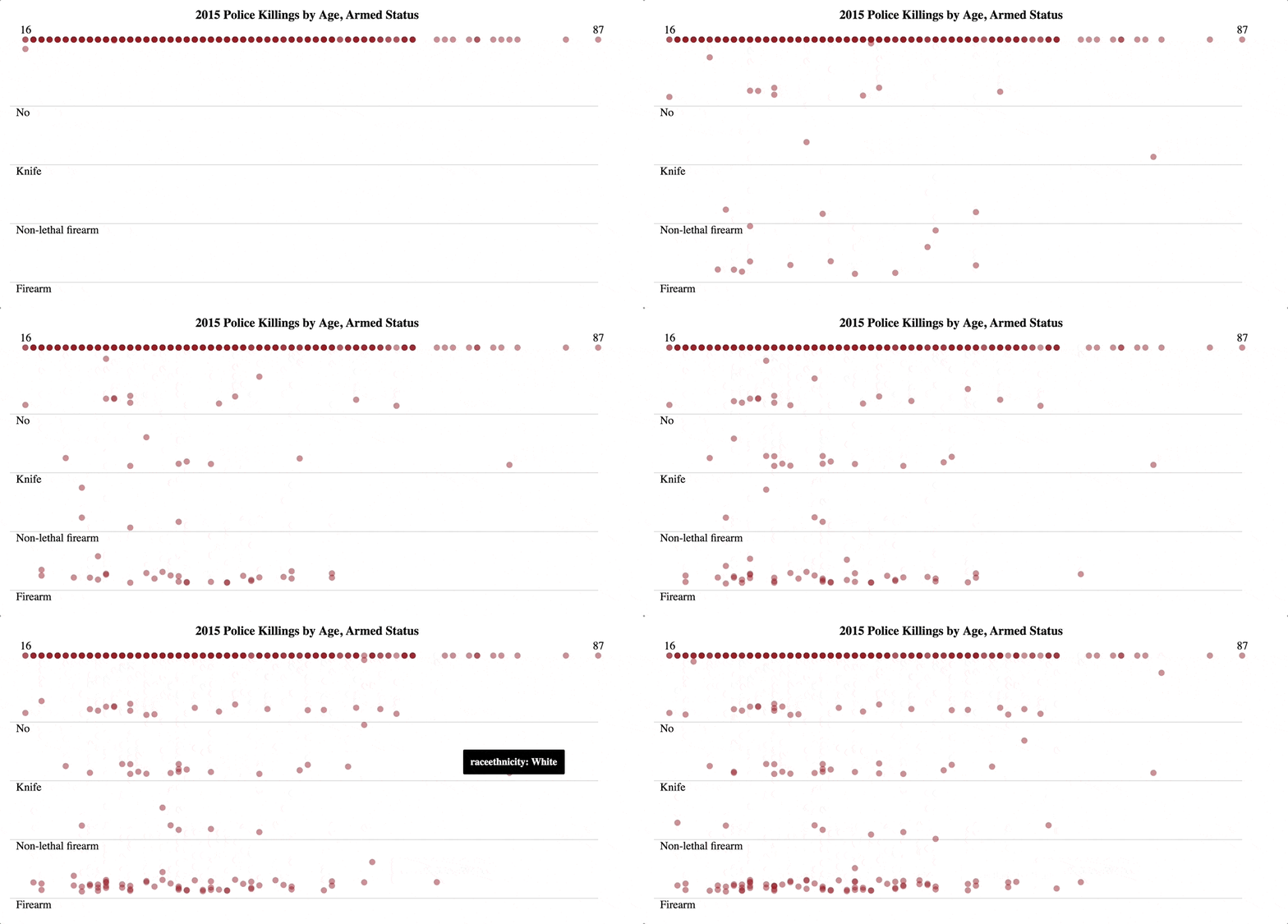
drip_settings adjusts the drip sequence, easing animation, jitter width, drip speed, and color. chart_settings controls the axes displays, font size, font family, and background color.

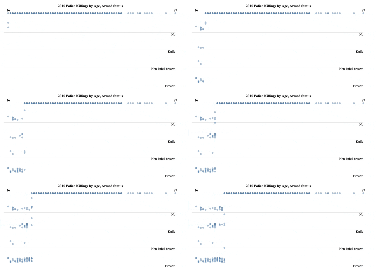
You can adjust the drip iteration by reordering the data frame:

pk %>% 
  arrange(age) %>% 
  d3rain(age, armed, toolTip = raceethnicity, title = "2015 Police Killings by Age, Armed Status") %>% 
  drip_settings(dripSequence = 'iterate',
                ease = 'linear',
                jitterWidth = 25,
                dripSpeed = 500,
                dripFill = 'steelblue') %>% 
  chart_settings(fontFamily = 'times',
                 yAxisTickLocation = 'left')

Rain Histograms

Create rain histograms with d3rain_hist and the accompanying functions:

d <- readr::read_csv("https://raw.githubusercontent.com/babeheim/citation-gates/master/citation-data-simulated.csv") %>% 
  rename(Downloaded = downloaded, 
         Contacted = contacted, 
         Replied = reply_received, 
         Received = data_received) %>% 
  mutate(Total = TRUE,
         `Downloaded and Received` = case_when(
           Downloaded ~ TRUE,
           Received ~ TRUE,
           TRUE ~ FALSE)
         ) 

d %>% 
  d3rain_hist(x = year, 
              levels = c("Total", "Contacted", "Replied", "Downloaded and Received"), 
              title = "Citation Statuses, 1960-2019") %>% 
  hist_chart_settings(annotations = c("Total Sample: 560", "475 (95%)", "309 (65%)", "147 (26%)"),
                      levelLabelLocation = "right") %>% 
  hist_drip_settings(colors = c("black", "forestgreen", "orange", "firebrick"),
                     transitionIntervals = 2500,
                     dripSpeed = 300)

Future Work

• Additional drip behaviors (e.g. by group)
• Conditional fill colors