Quickstart

Installation

import Pkg
Pkg.add("FlexiChains")

Obtaining a chain

MCMC sampling with Turing.jl or ParallelMCMC.jl returns a FlexiChain by default:

using Turing, FlexiChains
@model function f()
    x ~ Normal()
    y ~ Poisson(3.0)
    z ~ MvNormal(zeros(2), I)
end
model = f()
chain = sample(model, MH(), MCMCThreads(), 1000, 3)

╭─FlexiChain (1000 iterations, 3 chains) ───────────────────────────────╮
│ ↓ iter  = 1:1000                                                      │
│ → chain = 1:3                                                         │
│                                                                       │
│ Parameters (3) ── VarName                                             │
│  Float64          x                                                   │
│  Int64            y                                                   │
│  Vector{Float64}  z (2,)                                              │
│                                                                       │
│ Extras (4)                                                            │
│  Bool     accepted                                                    │
│  Float64  logprior, loglikelihood, logjoint                           │
╰───────────────────────────────────────────────────────────────────────╯

You can also construct a FlexiChain from a variety of other sources, including Pigeons.jl, Stan CSV files, PosteriorDB.jl, an MCMCChains.Chains object, or a matrix of DynamicPPL.VarNamedTuples or DynamicPPL.ParamsWithStats.

A quick primer on the data structure

A FlexiChain{T} stores data for parameters of type T, along with extras of any type which represent per-iteration metadata such as log densities.

Broadly speaking, a FlexiChain can be thought of as a dictionary mapping Union{Parameter{<:T},Extra} to niters x nchains matrices of samples. Each matrix can have a different element type, which allows FlexiChains to store samples as their original types (e.g. Int or Vector) rather than flattening and converting everything to Float64.

The most common types T are Symbol and AbstractPPL.VarName. The respective chain types are aliased to SymChain and VNChain.

Indexing

Indexing into a FlexiChain returns a DimMatrix from the DimensionalData.jl package, which behaves exactly like an ordinary Matrix but additionally carries more information about its dimensions.

chain[@varname(x)]              # -> (niters x nchains)     DimMatrix{Float64}
chain[@varname(y)]              # -> (niters x nchains)     DimMatrix{Int}
chain[@varname(z)]              # -> (niters x nchains)     DimMatrix{Vector{Float64}}
chain[@varname(z); stack=true]  # -> (niters x nchains x 2) DimArray{Float64} 

If you have a VNChain, you can access sub-components of parameters by specifying the appropriate VarName. Here z is a 2-dimensional vector, so accessing either z[1] or z[2] gives us scalars:

chain[@varname(z[1])] # -> (niters x nchains) DimMatrix{Float64}

You can index with Symbols, as long as it can be unambiguously resolved to a parameter or extra:

chain[:y]         # -> (niters x nchains) DimMatrix{Int}
chain[:logjoint]  # -> (niters x nchains) DimMatrix{Float64}

You can additionally subset iterations / chains using iter or chain keyword arguments:

chain[@varname(x), iter=101:End, chain=2]

(note that with keyword arguments you have to use End instead of end).

See the full guide to indexing for more.

Statistics

Quick and dirty summary stats can be obtained with:

ss = summarystats(chain)

This produces a FlexiSummary object with mean, standard deviation, Monte Carlo standard error, effective sample size, R-hat, and quantiles for each key:

╭─FlexiSummary (9 statistics) ──────────────────────────────────────────╮
│   iter    collapsed                                                   │
│   chain   collapsed                                                   │
│ ↓ stat  = [mean, std, mcse, ess_bulk, ess_tail, rhat, q5, q50, q95]   │
│                                                                       │
│ Parameters (4) ── VarName                                             │
│  Float64  x, y, z[1], z[2]                                            │
│                                                                       │
│ Extras (4)                                                            │
│  Float64  accepted, logprior, loglikelihood, logjoint                 │
│                                                                       │
│ Summary                                                               │
│   param     mean     std    mcse   ess_bulk   ess_tail    rhat  …     │
│       x  -0.0033  1.0190  0.0189  2888.7897  2657.3833  0.9998  …     │
│       y   2.9520  1.7255  0.0323  2869.7379  2988.1386  1.0002  …     │
│    z[1]  -0.0345  0.9956  0.0186  2863.4554  2624.3254  1.0000  …     │
│    z[2]   0.0267  1.0054  0.0181  3071.3115  2977.7340  1.0005  …     │
╰───────────────────────────────────────────────────────────────────────╯

You can index into this much like a FlexiChain:

ss[@varname(x), stat=:mean]  # mean of `x`

Or you can compute statistics directly with individual functions:

mean(chain)              # just the mean for all variables
mean(chain)[@varname(x)] # -> Float64
mean(chain; dims=:iter)  # take the mean over iterations only

See the full guide to summarising for more.

Plotting

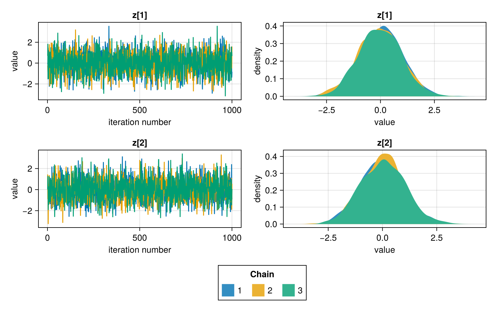
FlexiChains contains extensive functionality for visualising chains with Makie.jl and Plots.jl. Most of the effort has been focused on the Makie backend, and we recommend using this first.

using CairoMakie
plot(chain)                    # trace + densities for all parameters
plot(chain; pool_chains=true)  # combine samples from all chains
plot(chain, [@varname(z)])     # z[1] and z[2] only

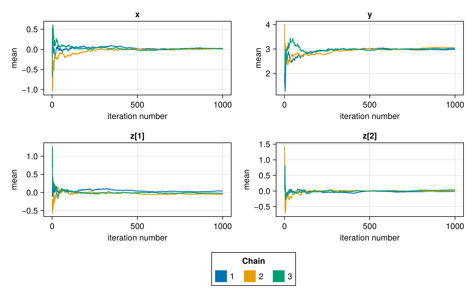
Specialised MCMC plots are namespaced under the FlexiChains.Makie module:

import FlexiChains.Makie as FM
FM.meanplot(chain; layout=(2, 2)) # Running mean plot, with custom grid layout

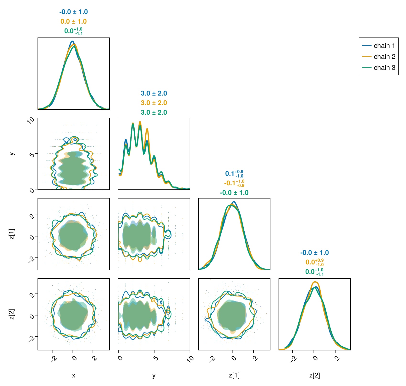
Pair plots can be generated with the PairPlots.jl extension:

using PairPlots
pairplot(chain)

The interface to Plots.jl is similar:

using StatsPlots
plot(chain)

import FlexiChains.Plots as FP
FP.meanplot(chain; layout=(2, 2))

StatsPlots.corner(chain)

See the full guide to plotting for more.