Development version:

August 21, 2026 · View on GitHub

##### Development version 1.2.1 (2026-08-14) ##### CRAN version 1.2.0 (2026-06-16)

GTFSwizard is a set of tools for creating, exploring, and manipulating General Transit Feed Specification (GTFS) files in R.

Its main purpose is to give researchers and practitioners a straightforward way to explore and simulate changes within GTFS files, which represent public transportation schedules and geographic data. The package lets users filter data by routes, trips, stops, and time, generate spatial visualizations, and analyze transit networks, including headways, dwell times, route frequencies, travel times, corridors, and hubs. Functions are also available to delay, change the speed of, split, and merge trips and feeds. This is ongoing work, with new features planned.

Installation

The development version is 1.2.1. The CRAN version is 1.2.0.

# CRAN version:
install.packages("GTFSwizard")
library(GTFSwizard)

# Development version:
install.packages('remotes') # if not already installed
remotes::install_github('OPATP/GTFSwizard@main')
library(GTFSwizard)

Documentation

The package website organizes the documentation by workflow:

Getting started: create, read, inspect, and export a feed.
Service analysis: service patterns, observational units, indicators, plots, corridors, and hubs.
Filtering and editing: build reproducible service scenarios while preserving the source feed.
Interactive dashboard: filter, inspect, edit, and export a feed with explore_gtfs().
Function reference: help pages grouped by task.

Basics

Use read_gtfs() to read an existing feed, as_wizardgtfs() to convert a GTFS list, and create_gtfs() to build and validate a feed from data frames. Each function returns a wizardgtfs object.

library(GTFSwizard)

gtfs <- GTFSwizard::read_gtfs('path-to-gtfs.zip') # or
gtfs <- GTFSwizard::as_wizardgtfs(gtfs_obj)

created_gtfs <- GTFSwizard::create_gtfs(
  agency = data.frame(
    agency_id = "A", agency_name = "Demo Transit",
    agency_url = "https://example.com",
    agency_timezone = "America/Fortaleza"
  ),
  routes = data.frame(
    route_id = "R1", agency_id = "A", route_short_name = "1",
    route_long_name = "Central", route_type = 3
  ),
  trips = data.frame(route_id = "R1", service_id = "WK", trip_id = "T1"),
  stop_times = data.frame(
    trip_id = "T1", arrival_time = c("08:00:00", "08:10:00"),
    departure_time = c("08:00:00", "08:10:00"),
    stop_id = c("S1", "S2"), stop_sequence = 1:2
  ),
  stops = data.frame(
    stop_id = c("S1", "S2"), stop_name = c("First", "Second"),
    stop_lat = c(-3.73, -3.74), stop_lon = c(-38.52, -38.53)
  ),
  calendar = data.frame(
    service_id = "WK", monday = 1, tuesday = 1, wednesday = 1,
    thursday = 1, friday = 1, saturday = 0, sunday = 0,
    start_date = "20260101", end_date = "20261231"
  )
)

summary(for_bus_gtfs)
# <summary.wizardgtfs>
#   Agency: ETUFOR
#   Service: 2019-09-13 to 2021-12-13 (823 active dates)
#   345 routes; 85410 trips; 4676 stops; 675 shapes
#   Median consecutive-stop spacing: 268.2 m
#
# Tables:
#          agency        calendar  calendar_dates fare_attributes      fare_rules 
#               1               3               6               2             345 
#          routes          shapes      stop_times           stops           trips 
#             345          125776         2659737            4676           85410

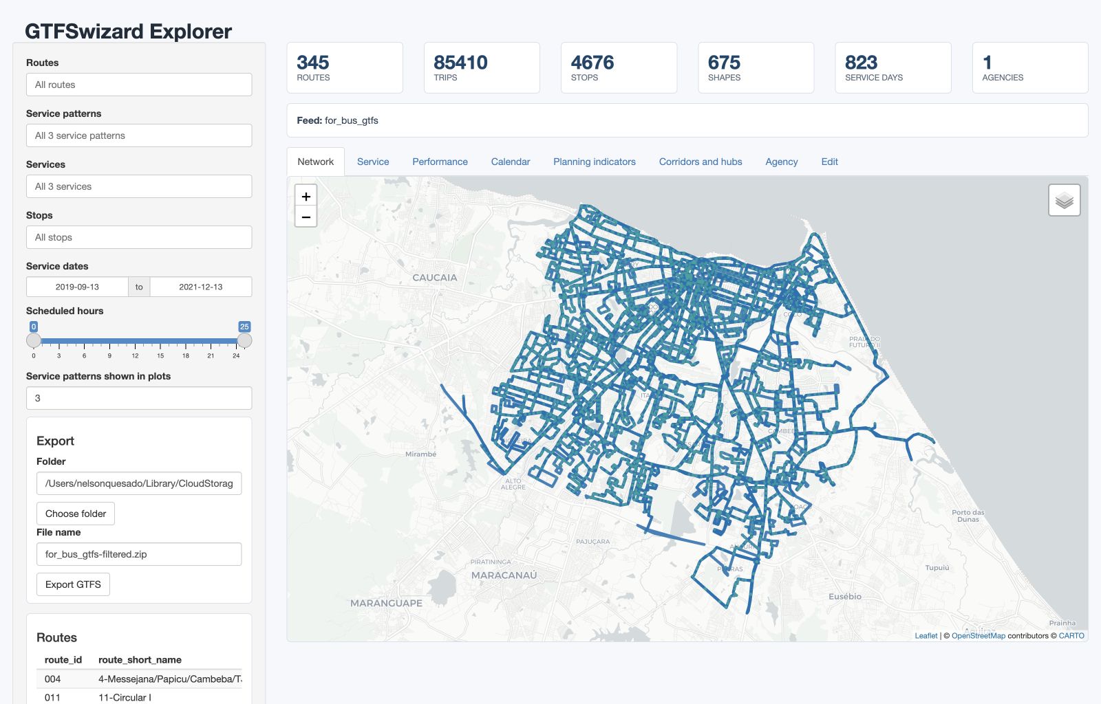
explore_gtfs() opens an interactive dashboard with maps and planning and operational views. Omit the argument to choose a GTFS .zip file in a browse window.

GTFSwizard::explore_gtfs(for_bus_gtfs)
GTFSwizard::explore_gtfs()

GTFSwizard interactive dashboard showing the transit network

Service Patterns

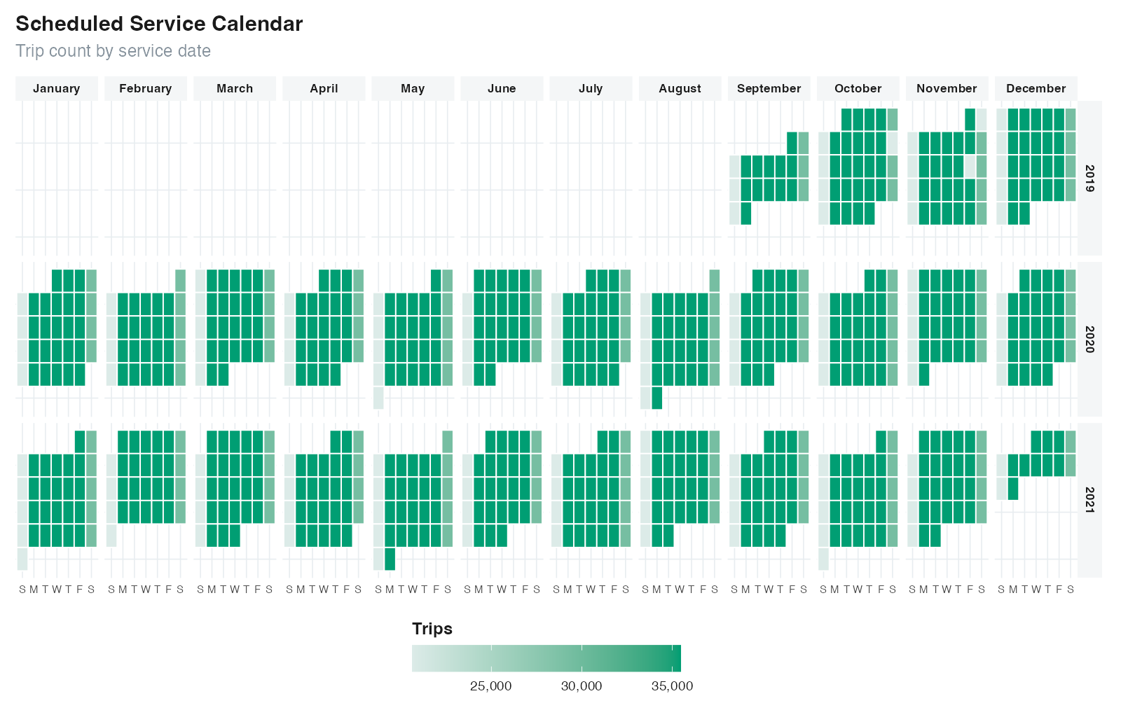
The concept of a service_pattern in GTFSwizard helps address a common limitation of GTFS: it does not identify recurring combinations of services active on a date. A pattern is the exact set of service_id values operating on a calendar date, independent of route.

In wizardgtfs objects, the dates_services table is an extended feature that consolidates dates and associated service_ids into a single, organized table. This table is not standard in typical GTFS files but is added specifically in wizardgtfs objects. The dates_services table is structured so that each date is associated with a list of service_ids representing the transit services operating on that specific day. Essentially, each unique list of service_ids observed across dates defines a distinct service pattern. It is common to observe at least 3 service patterns: weekdays, saturdays and sundays. Dates inside the feed calendar range with no active services are treated as an explicit empty service set: trip counts are 0, and the calendar-level pattern is labeled "No service".

Structure of dates_services: Each date in the dates_services table has an associated list of service_ids, capturing the set of services active on that particular day.
Defining Service Patterns: A unique service_pattern is identified by a unique combination of service_ids operating on a given date. For instance, if two dates share the exact same service_ids, they are considered part of the same service_pattern.
No-service dates: A date with no active service_ids is represented as the "No service" pattern in calendar-level outputs and by get_servicepattern() with service_id = NA. It is not a trip-bearing pattern and cannot be used with filter_servicepattern().

You can check service_pattern using the get_servicepattern() function.

``$ \text{r} \text{GTFSwizard}::\text{get_servicepattern}(\text{for_bus_gtfs})

\text{A} \text{tibble}: 3 \times 3

\text{service_id} \text{service_pattern} \text{pattern_frequency}

<\text{chr}> <\text{chr}> <\text{int}>

#1 \text{U} \text{servicepattern}-1 586 #2 \text{D} \text{servicepattern}-2 121 #3 \text{S} \text{servicepattern}-3 116 $``

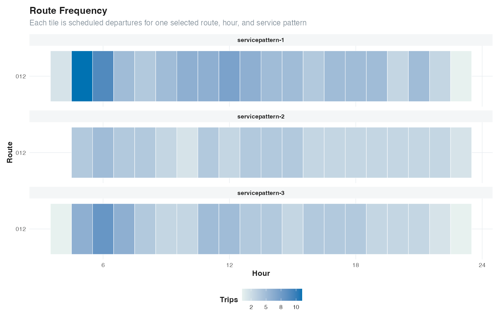
Most analytical functions account for service patterns, including get_frequency() and plot_routefrequency(). Patterns are ordered from most frequent (a useful typical-day default) to less frequent, and route-frequency plots compare the represented patterns.

GTFSwizard::get_frequency(for_bus_gtfs, method = "by_route")
## A tibble: 1,763 × 5
#  route_id direction_id service_pattern  pattern_frequency daily.frequency
#  <chr>           <dbl> <chr>                        <int>           <int>
#1 004                 0 servicepattern-1               586              22
#2 004                 1 servicepattern-1               586              23
#3 011                 1 servicepattern-1               586              95
#4 011                 1 servicepattern-2               121              43
#5 011                 1 servicepattern-3               116              73
#6 012                 0 servicepattern-1               586             102
## ℹ 1,757 more rows
## ℹ Use `print(n = ...)` to see more rows

GTFSwizard::plot_routefrequency(for_bus_gtfs, route = for_bus_gtfs$routes$route_id[3])

Scheduled route frequency by service pattern

You can use plot_calendar() to check the number of trips along the calendar and get a better sense of the service_pattern rationale. Dates without active service appear as 0 trips in trip-count mode and as "No service" in service-pattern mode.

GTFSwizard::plot_calendar(for_bus_gtfs, facet_by_year = TRUE)

Exploring

Frequency, headways, dwell times, speeds, durations, distances, fleet requirements, first departures, corridors, and hubs can be calculated directly from the schedule. Several functions support aggregation methods such as by_trip, by_route, by_hour, and detailed; see each function's help page for its exact observational unit.

GTFSwizard::get_headways(for_bus_gtfs, method = 'by_hour')
## A tibble: 73 × 5
#   hour service_pattern  pattern_frequency headway_minutes valid_trips
#  <dbl> <chr>                        <int>           <dbl>       <int>
#1     0 servicepattern-1               586            11.6           8
#2     0 servicepattern-2               121            11.6           8
#3     0 servicepattern-3               116            11.6           8
#4     1 servicepattern-1               586            64.4          32
#5     1 servicepattern-2               121            64.4          32
#6     1 servicepattern-3               116            64.4          32
## ℹ 67 more rows
## ℹ Use `print(n = ...)` to see more rows

GTFSwizard::get_durations(for_bus_gtfs, method = 'detailed', trips = 'all')
GTFSwizard::get_distances(for_bus_gtfs, method = 'by_trip', trips = 'all')
GTFSwizard::get_distances(for_bus_gtfs, method = 'by_route', trips = 'all')
GTFSwizard::get_speeds(for_bus_gtfs, method = 'by_route', trips = 'all')
GTFSwizard::get_fleet(for_bus_gtfs, method = 'peak')
GTFSwizard::get_1stdeparture(for_bus_gtfs)

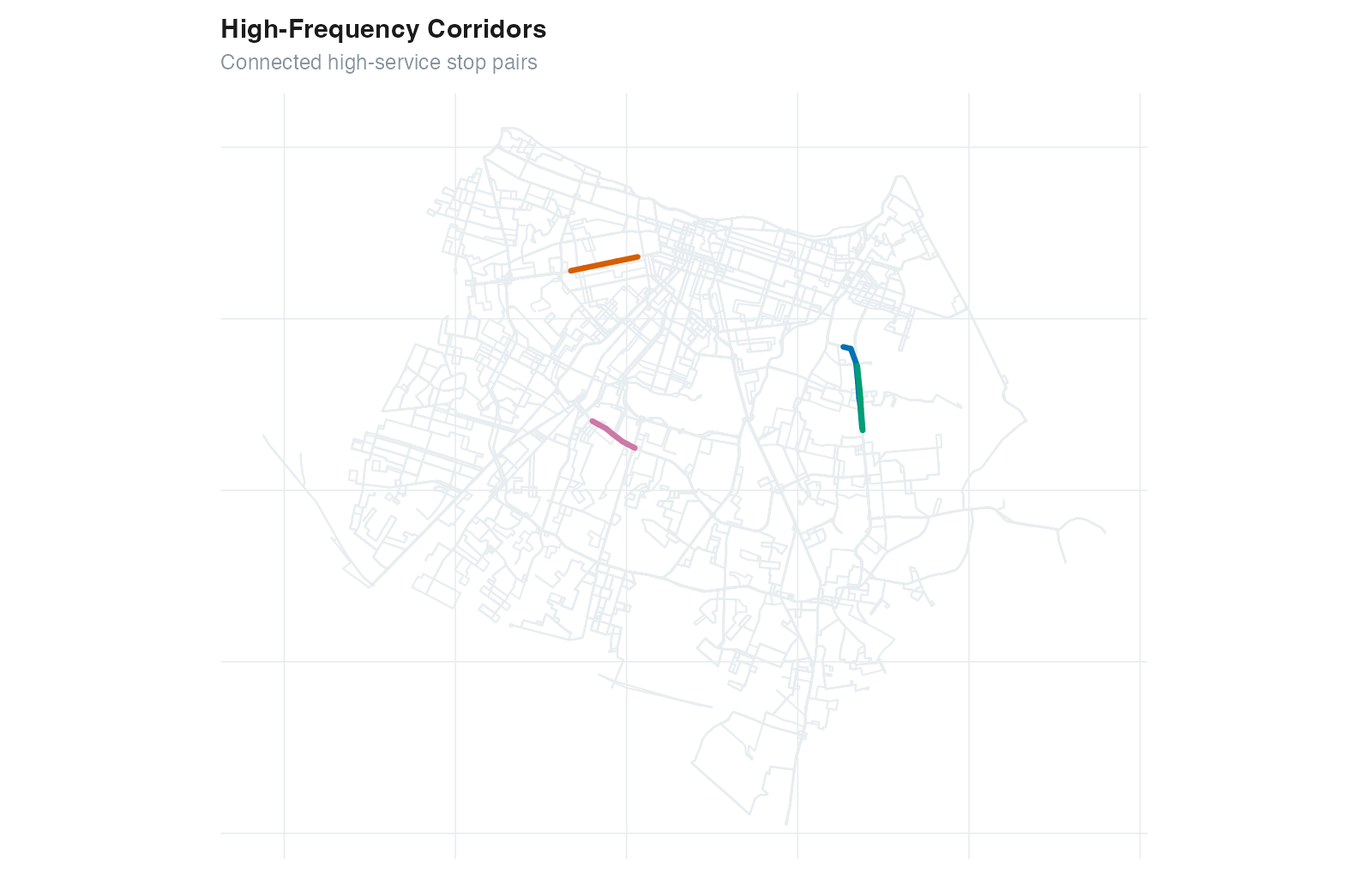
Corridors and hubs are simplified representations of critical links and nodes on transit networks.

Corridors: get_corridor() retrieves and plot_corridor() visualizes high-density transit sections.

GTFSwizard::get_corridor(for_bus_gtfs, i = .01, min_length = 1500)
# Simple feature collection with 4 features and 4 fields
# Geometry type: MULTILINESTRING
# Dimension:     XY
# Geodetic CRS:  WGS 84
# # A tibble: 4 × 5
#   corridor   stop_id   trip_id       length geometry
#   <chr>      <list>    <list>         <dbl> <MULTILINESTRING [°]>
# 1 Corridor 1 <chr [7]> <chr [3,429]>  2851. ((-38.48122 -3.781901, ...)
# 2 Corridor 2 <chr [5]> <chr [2,504]>  2214. ((-38.54677 -3.731971, ...)
# 3 Corridor 3 <chr [5]> <chr [3,470]>  2089. ((-38.48102 -3.782528, ...)
# 4 Corridor 4 <chr [7]> <chr [3,104]>  1635. ((-38.55838 -3.780695, ...)

GTFSwizard::plot_corridor(for_bus_gtfs)

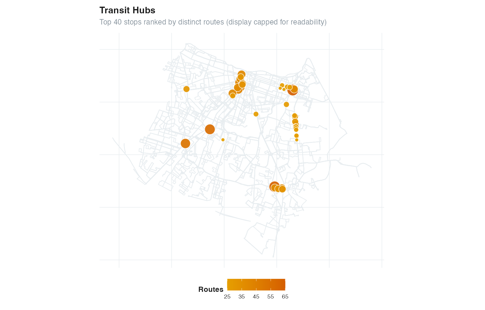
Hubs: get_hubs() retrieves and plot_hubs() visualizes high-connectivity transit stops.

GTFSwizard::get_hubs(for_bus_gtfs)
# Simple feature collection with 4676 features and 5 fields
# Geometry type: POINT
# # A tibble: 4,676 × 6
#   stop_id trip_id        route_id   n_trip n_routes geometry
#   <chr>   <list>         <list>      <int>    <int> <POINT [°]>
# 1 6079    <chr [14,745]> <chr [65]>  14745       65 (-38.48476 -3.738568)
# 2 4030    <chr [6,405]>  <chr [62]>   6405       62 (-38.50203 -3.830385)
# 3 6083    <chr [15,578]> <chr [56]>  15578       56 (-38.56358 -3.775878)
# 4 5822    <chr [14,364]> <chr [52]>  14364       52 (-38.58683 -3.789329)
# 5 1717    <chr [4,252]>  <chr [43]>   4252       43 (-38.5345 -3.735906)
# 6 6449    <chr [4,252]>  <chr [43]>   4252       43 (-38.53651 -3.738107)
## ℹ Use `print(n = ...)` to see more rows

GTFSwizard::plot_hubs(for_bus_gtfs)

Map of transit hubs sized by route connectivity

Filtering

Filtering tools allow GTFS data to be restricted by service patterns, dates, service IDs, route IDs, trip IDs, stop IDs, and time ranges. These filter_ functions retain the relevant records and their GTFS relationships.

filter_servicepattern(): Filter by specified active service patterns. Defaults to the most frequent active pattern (typical day) if none is provided. The "No service" pattern describes calendar days without trips and is not accepted by this filter.
filter_date(): Filter data by specific dates, returning only services active on those dates.
filter_service(): Filter by specific service IDs to retain.
filter_route(): Filter by route ID. Set keep = TRUE to retain specified routes or keep = FALSE to exclude them.
filter_trip(): Filter by trip ID. Set keep = TRUE to retain specified trips or keep = FALSE to exclude them.
filter_stop(): Keep stop calls at the requested stop IDs. Trips may remain partial, which supports route and network experiments.
filter_time(): Keep stop calls inside a specified time range (from and to). Trips that cross the time boundary remain as partial trips.

# Filter by service pattern
filtered_gtfs <- GTFSwizard::filter_servicepattern(for_bus_gtfs, "servicepattern-2")

# Filter by specific date
filtered_gtfs <- GTFSwizard::filter_date(for_bus_gtfs, "2021-02-10")

# Filter by route ID, retaining only specified routes
filtered_gtfs <- GTFSwizard::filter_route(for_bus_gtfs, for_bus_gtfs$routes$route_id[1:2])

# Filter by trip ID, excluding specified trips
filtered_gtfs <- GTFSwizard::filter_trip(for_bus_gtfs, for_bus_gtfs$trips$trip_id[1:2], FALSE)

# Filter by time range
filtered_gtfs <- GTFSwizard::filter_time(gtfs = for_bus_gtfs, "06:30:00", "10:00:00")

# Spatial filter using filter_stop
spatial.filter <- GTFSwizard::get_shapes_sf(for_bus_gtfs$shapes)

stops <- sf::st_filter(GTFSwizard::get_stops_sf(for_bus_gtfs$stops),
                       spatial.filter) |>
          dplyr::pull(stop_id)

filtered_gtfs <- GTFSwizard::filter_stop(for_bus_gtfs, stops)

Selecting and Grouping

selection() records a subset or grouping without removing any GTFS rows. Bare columns create groups in a style similar to dplyr::group_by(), while logical expressions restrict the records represented by the selection metadata.

# One group for each route and direction
grouped_gtfs <- GTFSwizard::selection(
  for_bus_gtfs,
  route_id,
  direction_id
)

# Group selected routes without modifying the original GTFS tables
selected_gtfs <- GTFSwizard::selection(
  for_bus_gtfs,
  route_id,
  route_id %in% for_bus_gtfs$routes$route_id[1:3]
)

attr(selected_gtfs, "selection")$groups
selected_gtfs <- GTFSwizard::unselection(selected_gtfs)

Visualizing

GTFSwizard provides consistent static plots for network supply and scheduled operations. Plot subtitles and axes state the observational unit represented.

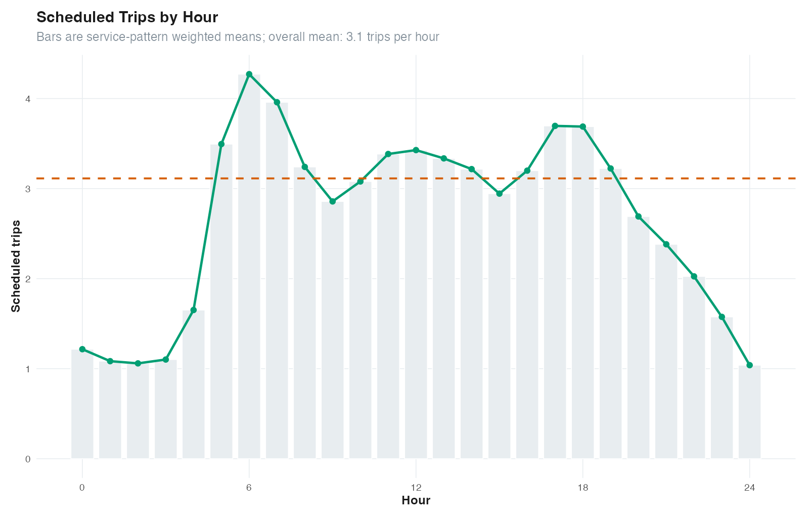
System Frequency by Hour: plot_frequency() shows the distribution of trip frequencies by hour, with hourly and overall averages to highlight peak service times.

GTFSwizard::plot_frequency(for_bus_gtfs)

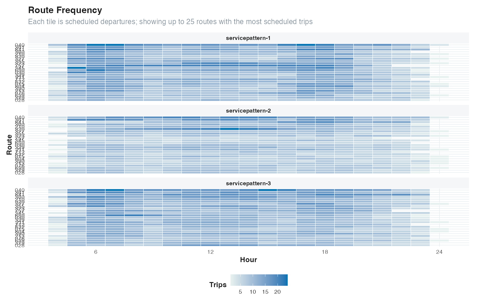
Route Frequency by Hour: plot_routefrequency() displays a tile plot where fill is the number of scheduled trips by route, hour, and service pattern. Use top_n to keep large feeds readable.

GTFSwizard::plot_routefrequency(for_bus_gtfs, route = for_bus_gtfs$routes$route_id[4:5])

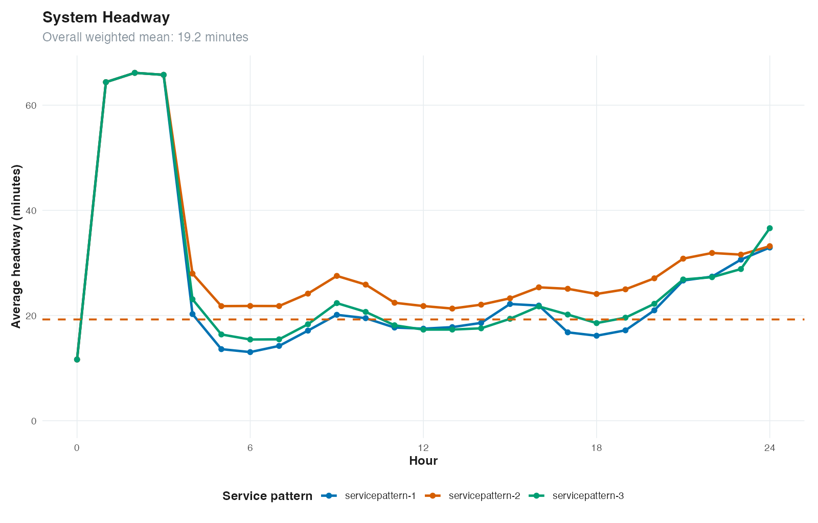
System Average Headway by Hour: plot_headways() shows average time between trips, highlighting hourly and overall headways to visualize service intervals.

GTFSwizard::plot_headways(for_bus_gtfs)

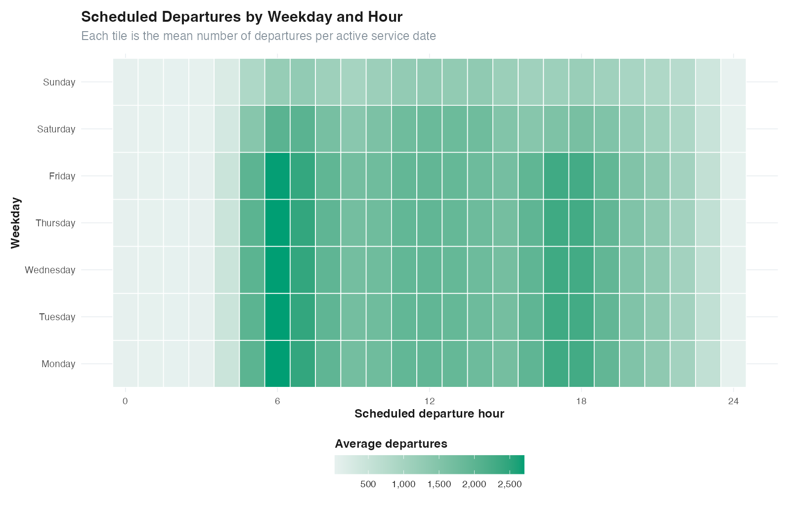
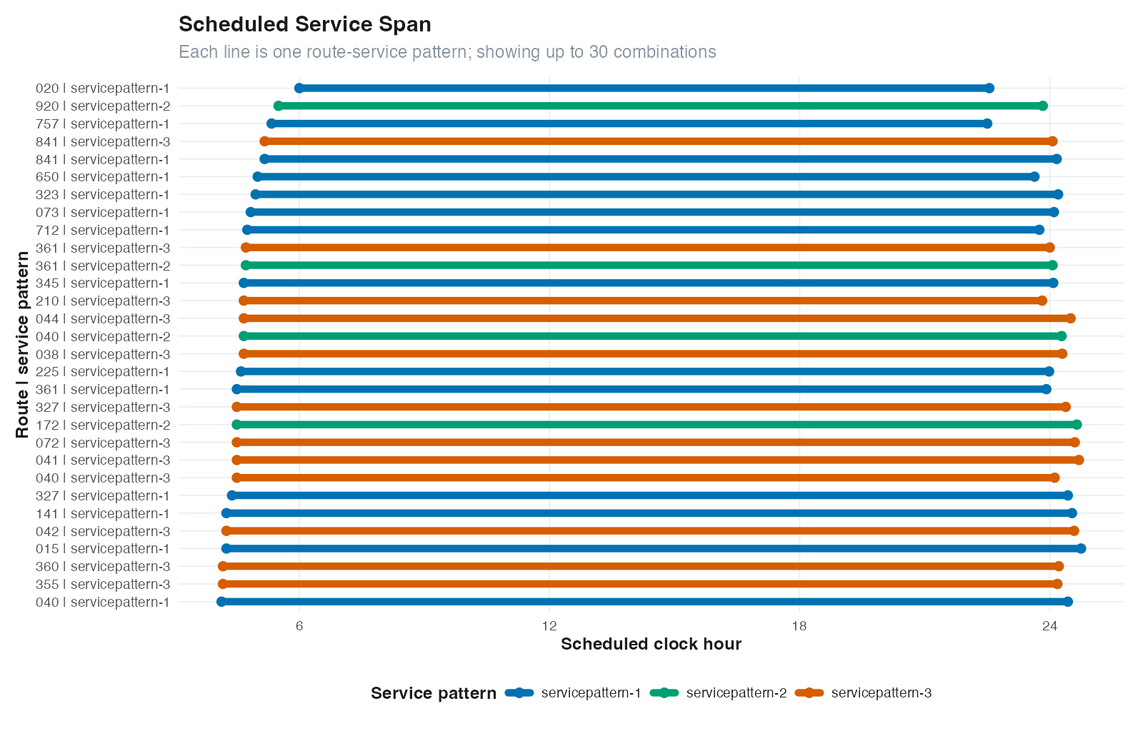
Planning views: plot_servicespan() shows the first departure and final arrival for each route-service pattern, plot_serviceheatmap() summarizes departures by weekday and hour, plot_routeduration() shows scheduled trip-duration distributions, and plot_servicesupply() reports scheduled vehicle-hours.

GTFSwizard::plot_servicespan(for_bus_gtfs)
GTFSwizard::plot_serviceheatmap(for_bus_gtfs)
GTFSwizard::plot_routeduration(for_bus_gtfs)
GTFSwizard::plot_servicesupply(for_bus_gtfs)

Scheduled departures by weekday and hour

Editing

GTFSwizard provides functions to edit GTFS data directly. The delay_trip() function allows users to apply a delay to specific trips. The split_trip() function divides a trip into valid consecutive parts. Trips can be split into split + 1 approximately equal parts, or at selected internal stop IDs using the stops argument. This can be useful for analyzing partial routes or for simulating route adjustments. The edit_speed() function adjusts the travel speeds between stops in a GTFS dataset by modifying trip durations based on a specified speed multiplier. It allows selective adjustments for specific trips and stops or applies changes globally. The set_dwelltime() function overwrites selected dwell times while retaining arrival at each edited stop and shifting downstream times. The trip end time may therefore change. The edit_dwelltime() function scales selected dwell times and applies the same downstream propagation. The merge_gtfs() function combines two GTFS files, allowing for the integration of distinct GTFS datasets into a single dataset.

# Delay trips by 5 minutes (300 seconds)
delayed_gtfs <- GTFSwizard::delay_trip(for_bus_gtfs, trip = for_bus_gtfs$trips$trip_id[1:2], duration = 300)

# Split a trip in 3 sections (2 splits)
split_gtfs <- GTFSwizard::split_trip(for_bus_gtfs, trip = for_bus_gtfs$trips$trip_id[1:2], split = 2)

# Split a trip at selected stop IDs
split_at_stop_gtfs <- GTFSwizard::split_trip(for_bus_gtfs, trip = for_bus_gtfs$trips$trip_id[1], stops = for_bus_gtfs$stop_times$stop_id[2])

# Merge two GTFS files into one
merged_gtfs <- GTFSwizard::merge_gtfs(for_bus_gtfs, for_rail_gtfs)

# Double the speed of all trips
faster_gtfs <- GTFSwizard::edit_speed(for_rail_gtfs, factor = 2)

# Set and edit dwell times for specific trips
gtfs <- set_dwelltime(for_rail_gtfs,                            
                   trips = for_rail_gtfs$trips$trip_id[1:100],
                   stops = for_rail_gtfs$stops$stop_id[1:20],
                   duration = 10)

gtfs <- edit_dwelltime(gtfs,                                    
                   trips = for_rail_gtfs$trips$trip_id[1:100],
                   stops = for_rail_gtfs$stops$stop_id[1:20],
                   factor = 1.5)

get_dwelltimes(gtfs, method = 'detailed')

Export a resulting feed with write_gtfs(), which writes a standard GTFS .zip archive to the requested path.

GTFSwizard::write_gtfs(for_bus_gtfs, 'path-to-file.zip')

Travel Time Matrix

GTFSwizard implements the tidytransit::raptor() algorithm that estimates travel time matrices from a wizardgtfs object and a few other arguments.

GTFSwizard::tidy_raptor(for_rail_gtfs, min_departure = '06:20:00', max_arrival = '09:40:00',
           dates = "2021-12-13", max_transfers = 2, keep = "all",
           stop_ids = '66')

Handling Geographic Data

GTFSwizard autodetects and reconstructs missing shape tables using the get_shapes() function. Variations of this function can create simple feature objects from stops or shapes tables, using get_stops_sf() or get_shapes_sf() functions, or standard GTFS shapes data frames from simple-feature shape objects using get_shapes_df(). Because get_shapes() reconstructs geometry from stop sequences, shapes created after filter_stop() or filter_time() describe only the retained partial trips.

gtfs <- for_bus_gtfs

gtfs$shapes <- NULL

gtfs$shapes
#NULL

gtfs <- GTFSwizard::get_shapes(gtfs)

GTFSwizard::get_shapes_sf(for_bus_gtfs$shapes)

GTFSwizard::get_stops_sf(for_bus_gtfs$stops)

The latlon2epsg() function determines the appropriate UTM (Universal Transverse Mercator) EPSG code for a given sf object based on its centroid's latitude and longitude. This can be very useful for conveniently geoprocessing data in meters.

GTFSwizard::latlon2epsg(get_shapes_sf(for_bus_gtfs)$shapes)

Objects

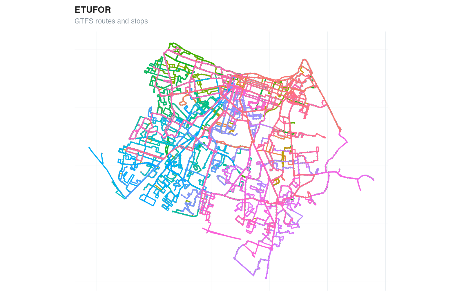
GTFSwizard features two toy examples, a small for_rail_gtfs wizardgtfs object, and a rather bigger for_bus_gtfs wizardgtfs object. They are real GTFS samples, the first being the urban subway system, and the second one the regular bus system; both for the city of Fortaleza, Brazil, on the 2020's.

gtfs <- GTFSwizard::for_bus_gtfs

plot(gtfs)

Applications

The functions described facilitate the analysis, simulation, and evaluation of public transportation systems. They assist the replication of real-world transit interventions, enabling researchers, planners, and policymakers to test and refine system modifications in a controlled and efficient manner. Key applications are outlined below along with their potential uses in addressing typical challenges and opportunities in public transit systems.

Bus Rapid Transit (BRT) and Exclusive Lanes: BRT systems often rely on exclusive corridors to reduce travel times and enhance reliability. Using edit_speed(), users can represent changes towards smaller travel times on these corridors by adjusting travel speeds. In addition, edit_dwelltime() allows the representation of optimized boarding and alighting processes, reflecting reduced dwell times at stations due to level boarding, pre-payment mechanisms, or increased operational efficiency;
Frequency Modifications: Frequency adjustments are among the most common transit interventions. By using filter_trip() to select trips to be doubled, delay_trip() to change its first departure_time, and merge_gtfs() to add them to the original GTFS, users can represent increased frequencies, reflecting higher service levels. Conversely, filter_trip can be used to reduce service frequencies, allowing for the evaluation of cost-saving measures or temporary schedule adjustments;
Route Segmentation and Partial Adjustments: With split_trip(), users can divide existing routes into smaller segments, enabling partial route adjustments. This is particularly relevant in studies assessing the feasibility of feeder services, route rationalization, or service redundancy elimination.
Express Services: Transit stops significantly influence travel times, operating costs, and network coverage. Using edit_dwelltime() and filter_stop() can subtract dwell times from total trip durations and remove unused stops, representing the introduction of express services.

Cheat Sheet

See the GTFSwizard cheat sheet for a compact guide to the main workflow: creating or reading feeds, selecting services, plotting operations, editing GTFS, exploring feeds interactively, and writing results.

Contributing

Contributions are welcome! To report a bug, suggest a feature, or contribute code, please use the repository’s Issues.

GTFSwizard mainly uses dplyr for data handling, sf for spatial operations, and ggplot2 for static visualization. shiny and leaflet are optional dependencies for explore_gtfs(). tidytransit, data.table, and hms are optional dependencies used only by tidy_raptor().

Citation

To cite package ‘GTFSwizard’ in publications use:

Quesado Filho, N. O.; Guimaraes, C. G. C.; de Oliveira Neto, F. M. (2026). GTFSwizard: Creating, Exploring and Manipulating GTFS Files. R package version 1.2.1. doi:10.32614/CRAN.package.GTFSwizard.

A BibTeX entry for LaTeX users is

  @Manual{quesado.guimaraes.oliveiraneto.2026,
    title = {GTFSwizard: Creating, Exploring and Manipulating GTFS Files},
    author = {N. O. {Quesado Filho} and C. G. C. {Guimaraes} and F. M. {de Oliveira Neto}},
    year = {2026},
    note = {R package version 1.2.1},
    url = {https://cran.r-project.org/package=GTFSwizard},
    doi = {10.32614/CRAN.package.GTFSwizard}}

QUESADO FILHO, N. de O.; GUIMARÃES, C. G. C.; OLIVEIRA NETO, F. M. de. GTFSwizard: a set of tools for exploring and manipulating general transit feed specification in R language. CONTRIBUCIONES A LAS CIENCIAS SOCIALES, [S. l.], v. 18, n. 1, p. e14620, 2025. DOI: 10.55905/revconv.18n.1-197.

QUESADO FILHO, N. O.; GUIMARAES, C. G. C. ; OLIVEIRA NETO, F. M. . How to use GTFSwizard R Package to Assess Transit Projects: Fortaleza's BR-116 Bus Rapid Transit System Proposal. In: 39º Congresso de Pesquisa e Ensino em Transportes, 2025, Goiânia. Anais do 39º Congresso de Pesquisa e Ensino em Transportes, 2025.

Acknowledgement

GTFSwizard is developed by Nelson Quesado, Caio Guimarães and Fco. Moraes at OPA-TP research group, Universidade Federal do Ceará.