README.md
July 26, 2026 · View on GitHub
SAX-VSM public code release




This code supports our publication:
Senin, Pavel and Malinchik, Sergey, SAX-VSM: Interpretable Time Series Classification Using SAX and Vector Space Model, Data Mining (ICDM), 2013 IEEE 13th International Conference on, pp.1175,1180, 7-10 Dec. 2013.
Also available in R and Python (saxpy).
Cross-implementation alignment
This Java code, the R/C++ (jmotif-R), and
the Python (saxpy) implementations are kept
aligned. As of 2.1.0 this build depends on the aligned jmotif-sax 2.0.1 from Maven Central, so
the SAX layer (population-std z-normalization, fractional PAA, Gaussian
breakpoints, on-breakpoint→symbol-above) matches the other two to
floating-point precision. The TF*IDF weight uses log1p term frequency,
ln(1 + tf), and a natural-log IDF, ln(N / df) — matching saxpy and
jmotif-R. (Earlier versions of this repo used the SMART 1 + ln(tf) / log10
scheme; a cross-implementation accuracy study over CBF, Gun_Point, Coffee, Beef,
OSULeaf and Adiac found log1p ties or beats SMART at the tuned operating point
on every dataset and wins more parameter points overall, so log1p is now
canonical across all three.) The IDF base (ln vs log10) is a uniform
per-word factor that cancels in the cosine similarity, so it never changes a
classification — only the printed weight magnitudes. The five TF variants shown
in §5.0 NOTES remain available in the source for experimentation.
Cross-language checks for the shared SAX layer (discord search, sliding-window SAX, RePair) and SAX-VSM classifier accuracy (CBF, Gun_Point) live in jmotif-conformance.
Our algorithm is based on the following work:
[1] Lin, J., Keogh, E., Wei, L. and Lonardi, S., Experiencing SAX: a Novel Symbolic Representation of Time Series. DMKD Journal, 2007.
[2] Salton, G., Wong, A., Yang., C., A vector space model for automatic indexing. Commun. ACM 18, 11, 613–620, 1975.
[3] Jones, D. R. , Perttunen, C. D., and Stuckman, B. E., Lipschitzian optimization without the lipschitz constant, Journal of Optimization Theory and Applications, vol. 79, no. 1, pp. 157–181, 1993
[4] The DiRect implementation source code is partially based on JCOOL.
0.0 In a nutshell
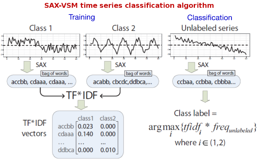
The proposed interpretable time series classification algorithm consists of two steps -- training and classification.
For training, labeled time series discretized with SAX via sliding window and "bag of words" constructed for each of the training classes (single bag per class). Processing bags with TFIDF yields a set of class-characteristic vectors -- one vector per class. Essentially, each element of that vector is a weighted discretized fragment of the input time series whose weight value reflects its "class-characteristic power" and the class specificity.
For classification, the unlabeled time series is discretized with sliding window-based SAX (exactly the same transform as for training) in order to transform it into a term frequency vector. Next, the cosine similarity computed between this vector and those constructed during training (i.e., vectors characterizing training classes). The unlabeled input time series assigned to a class with which the angle is smallest, i.e., the cosine value is largest. This is ltc.nnn schema in SMART notation.
Because it is easy to see which patterns contribute the most to the cosine similarity value, as well as to see which patterns have the highest weights after training, the algorithm naturally enables the interpretation of training and classification results.
The whole process is illustrated below:
1.0 Building
The code is written in Java and I use maven to build it. Version 2.1.0 depends on
jmotif-sax 2.0.1 from Maven Central:
$ mvn -P single -DskipTests package
The single profile assembles the fat jar:
$ mvn -P single -DskipTests package
[INFO] Scanning for projects...
[INFO] ------------------------------------------------------------------------
[INFO] Building sax-vsm 2.1.0
[INFO] ------------------------------------------------------------------------
...
[INFO] Building jar: target/sax-vsm-2.1.0.jar
[INFO] Building jar: target/sax-vsm-2.1.0-jar-with-dependencies.jar
[INFO] ------------------------------------------------------------------------
[INFO] BUILD SUCCESS
[INFO] ------------------------------------------------------------------------
[INFO] Total time:  7.xxx s
Drop -DskipTests to run the test suite as part of the build. The build produces two
artifacts: the thin target/sax-vsm-2.1.0.jar and the self-contained
target/sax-vsm-2.1.0-jar-with-dependencies.jar used in the examples below.
2.0 Running the classifier
Class SAXVSMClassifier is runnable from command line; running it without parameters prints usage help. The options are -train, -test, -w/--window_size (default 30), -p/--word_size (default 4), -a/--alphabet_size (default 3), --strategy one of [NONE, EXACT, MINDIST] (default EXACT), and --threshold (default 0.01). Here is a trace of running SAX-VSM with the Gun/Point dataset:
$ java -cp "target/sax-vsm-2.1.0-jar-with-dependencies.jar" net.seninp.jmotif.SAXVSMClassifier \
  -train src/resources/data/Gun_Point/Gun_Point_TRAIN -test src/resources/data/Gun_Point/Gun_Point_TEST \
  -w 33 -p 17 -a 15
12:34:56.001 [main] INFO net.seninp.jmotif.SAXVSMClassifier - trainData classes: 2, series length: 150
12:34:56.003 [main] INFO net.seninp.jmotif.SAXVSMClassifier -  training class: 2 series: 26
12:34:56.003 [main] INFO net.seninp.jmotif.SAXVSMClassifier -  training class: 1 series: 24
12:34:56.004 [main] INFO net.seninp.jmotif.SAXVSMClassifier - testData classes: 2, series length: 150
12:34:56.004 [main] INFO net.seninp.jmotif.SAXVSMClassifier -  test class: 2 series: 74
12:34:56.004 [main] INFO net.seninp.jmotif.SAXVSMClassifier -  test class: 1 series: 76
classification results: strategy EXACT, window 33, PAA 17, alphabet 15,  accuracy 0.98667,  error 0.01333
As of 2.0.1 the run log goes through SLF4J -- every line above except the
final classification results: line (plain stdout) is prefixed with
HH:MM:SS.mmm [main] INFO net.seninp.jmotif.SAXVSMClassifier - .
The -w 33 -p 17 -a 15 operating point used to report accuracy 1.00, error 0.00
in pre-2.0 releases. With the jmotif-sax 2.0.x SAX layer and the log1p TF·IDF
alignment (see Cross-implementation alignment above) it now reports
accuracy 0.98667, error 0.01333 -- a two-series shift, and the same numbers the
DiRect sampler's NONE strategy lands on in §3.0. The alignment dataset CBF, e.g.
-train src/resources/data/cbf/CBF_TRAIN -test src/resources/data/cbf/CBF_TEST -w 60 -p 8 -a 6,
classifies at accuracy 1.00, error 0.00.
3.0 Running the parameters sampler (optimizer)
Symbolic discretization with SAX -- the first step of our algorithm -- requires hyperparameters to be specified by the user. Unfortunately, their optimal selection is not trivial. We proposed to use Dividing Rectangles optimization scheme for accelerated selection of optimal parameter values.
The code implements the DiRect sampler which can be called from the command line (it is the main class of the fat jar, so java -jar runs it). The options are -wmin/-wmax (default 10/100), -pmin/-pmax (default 3/10), -amin/-amax (default 3/5), --hold_out (default 1), -i/--iter (default 1), and -b/--break (default 0.001). Below is the trace of running the sampler for the Gun/Point dataset. The series in this dataset have length 150, so I define the sliding window range as [10-150], PAA size as [5-75], and the alphabet [2-18]:
$ java -jar target/sax-vsm-2.1.0-jar-with-dependencies.jar \
  -train src/resources/data/Gun_Point/Gun_Point_TRAIN -test src/resources/data/Gun_Point/Gun_Point_TEST \
  -wmin 10 -wmax 150 -pmin 5 -pmax 75 -amin 2 -amax 18 --hold_out 1 -i 3
12:40:01.101 [main] INFO ... - trainData classes: 2, series length: 150
12:40:01.103 [main] INFO ... -  training class: 2 series: 26
12:40:01.103 [main] INFO ... -  training class: 1 series: 24
12:40:01.104 [main] INFO ... - testData classes: 2, series length: 150
12:40:01.104 [main] INFO ... -  test class: 2 series: 74
12:40:01.104 [main] INFO ... -  test class: 1 series: 76
12:40:01.110 [main] INFO ... - running sampling for NONE strategy...
@0.18	80	40	10
@0.04	80	17	10
...
 iteration: 0, minimal value 0.0 at 80, 40, 10
 iteration: 1, minimal value 0.0 at 80, 40, 10
 iteration: 2, minimal value 0.0 at 80, 40, 10
min CV error 0.00 reached at [80, 40, 10], [33, 17, 15], will use Params [windowSize=33, paaSize=17, alphabetSize=15, nThreshold=0.01, nrStrategy=NONE, cvError=0.0]
error 0.06,    strategy MINDIST, window 33, PAA 17, alphabet 15, (CV error 0.02)
error 0.02667, strategy EXACT,   window 33, PAA 17, alphabet 10, (CV error 0.00)
error 0.01333, strategy NONE,    window 33, PAA 17, alphabet 15, (CV error 0.00)
all done in # ~2394 ms
Each evaluated point is logged as @<error>\t<window>\t<paa>\t<alpha>,
each iteration prints a iteration: N, minimal value ... at w, p, a summary, and the
per-strategy result lines and all done in # ... ms close the run. Several parameter
combinations tie at the minimal CV error (here [80, 40, 10] and [33, 17, 15]); the
sampler breaks ties by choosing the set with the smallest sliding window. The NONE
optimum [33, 17, 15] lands at error 0.01333 -- the same point and number as the
direct §2.0 classifier run.
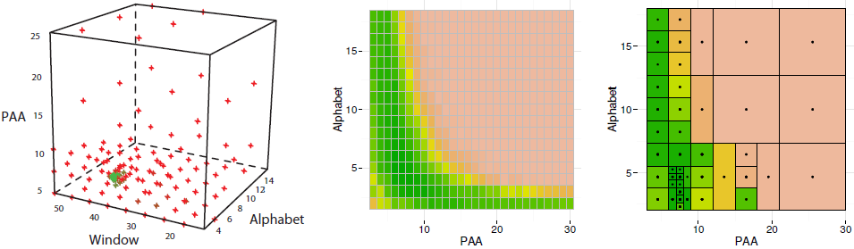
As shown in our work, DiRect provides a significant speed-up when compared with the grid search. Below is an illustration of DiRect-driven parameters optimization for SyntheticControl dataset. Left panel shows all points sampled by DiRect in the space PAA ∗ Window ∗ Alphabet: red points correspond to high error values while green points correspond to low error values in cross-validation experiments. Note the green points concentration at W=42 (where the optimal value is). Middle panel shows the classification error heat map obtained by a complete scan of all 432 points of the hypercube slice when W=42. Right panel shows the classification error heat map of the same slice when the parameters search optimized by DiRect, the optimal solution (P=8,A=4) was found by sampling of 43 points (i.e., 10X speed-up for the densely sampled slice).
4.0 Interpretable classification
The class named SAXVSMPatternExplorer prints the most significant class-characteristic patterns, their weights, and the time-series that contain those. The best_words_heat.R script allows to plot these. Here is an example for the Gun/Point data:
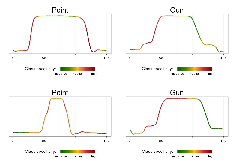
The highlighted time series ranges match distinctive class features: class Gun is characterized the most by articulated movements for prop retrieval and aiming, class Point is characterized by the ‘overshoot’ phenomenon and simpler (when compared to Gun) movement before aiming.
4.1 Unsupervised clustering
Classification merges all training series of a class into one bag per class. Clustering uses the same SAX-VSM tf·idf geometry but builds one vector per series (class:index labels) and groups them with k-means or hierarchical clustering. The facade is SAXVSMClustering in package net.seninp.jmotif.cluster.

Figure: CBF train sample (30 series) — single-linkage dendrogram on per-series tf·idf vectors (top) and the three canonical shapes (bottom). Generated with cbf_clustering_plots.R.
Clustering purity (fraction of series whose true class matches the plurality label in their assigned cluster) on bundled UCR train subsets at the same SAX parameters as §2.0:
| Dataset | Train series | k | Classifier test error | k-means purity | HC single purity (k-cut) |
|---|---|---|---|---|---|
| CBF | 30 | 3 | 0.00 (900 test) | 0.90 (furthest-first, seed 2) | 1.00 |
| Gun_Point | 50 | 2 | 0.0133 (150 test) | 0.86 (furthest-first, seed 21) | 0.52–0.56 (root cut)* |
*Gun_Point does not split cleanly at the dendrogram root; use k-means or a Dendrogram.partition(k) cut rather than the top merge alone. CBF is the better clustering demo: three shapes separate almost perfectly in tf·idf space (matching 100% classifier accuracy on the full test set).
Short Java tutorial (JUnit-style; data under src/resources/data/cbf/):
import java.util.List;
import java.util.Map;
import net.seninp.jmotif.cluster.*;
import net.seninp.jmotif.sax.NumerosityReductionStrategy;
import net.seninp.jmotif.text.Params;
import net.seninp.util.UCRUtils;

Map<String, List<double[]>> train =
    UCRUtils.readUCRData("src/resources/data/cbf/CBF_TRAIN");
Params params = new Params(60, 8, 6, 0.01, NumerosityReductionStrategy.EXACT);

Map<String, Map<String, Double>> tfidf = SAXVSMClustering.seriesTfidf(train, params);
Map<String, String> labels = SAXVSMClustering.seriesLabels(train);

// k-means (golden test: purity 0.90)
ClusterAssignments km =
    SAXVSMClustering.kMeans(tfidf, 3, KMeansInit.FURTHEST_FIRST, 2L);
double kmPurity = km.labelPurity(labels);

// hierarchical clustering + greedy 3-way cut (golden test: purity 1.00)
Dendrogram tree = SAXVSMClustering.hierarchical(tfidf, Linkage.SINGLE);
ClusterAssignments hc = tree.partition(3);
double hcPurity = hc.labelPurity(labels);
Golden tests: TestSAXVSMClustering. Reproduce the figure: Rscript src/resources/RCode/cbf_clustering_plots.R (requires jmotif-R).
Command-line clustering — class SAXVSMClusteringCLI; running without parameters prints usage. Options mirror the classifier SAX knobs plus -train, -k, -m/--method (kmeans or hierarchical), --linkage (single or complete), --init (random or furthest_first), --seed, and optional --newick_out. Example on CBF train:
$ java -cp "target/sax-vsm-2.1.0-jar-with-dependencies.jar" net.seninp.jmotif.cluster.SAXVSMClusteringCLI \
  -train src/resources/data/cbf/CBF_TRAIN -k 3 -w 60 -p 8 -a 6 --init furthest_first --seed 2
clustering results: method kmeans, strategy EXACT, window 60, PAA 8, alphabet 6, k 3, init furthest_first, seed 2, purity 0.90
  cluster 0 (n=7): {2=1, 3=6}
  cluster 1 (n=12): {1=10, 3=2}
  cluster 2 (n=11): {2=11}
Single-linkage hierarchical clustering with a 3-way partition:
$ java -cp "target/sax-vsm-2.1.0-jar-with-dependencies.jar" net.seninp.jmotif.cluster.SAXVSMClusteringCLI \
  -train src/resources/data/cbf/CBF_TRAIN -k 3 -m hierarchical --linkage single -w 60 -p 8 -a 6
clustering results: method hierarchical, strategy EXACT, window 60, PAA 8, alphabet 6, k 3, linkage single, purity 1.00
newick: (...)
Log lines go through SLF4J; the clustering results: line, per-cluster counts, and optional newick: line are plain stdout (same pattern as SAXVSMClassifier).
5.0 NOTES
The default choice for validating the best parameters on TEST data is the parameter set with the shortest sliding window. You may prefer another tie-break — for example, the point whose neighborhood has the highest density of sampled points.
The code implements five ways to compute TF (term frequency). As of 2.0.1 the log1p variant (first line) is the canonical/default, uncommented, choice and is the one aligned with saxpy and jmotif-R:
double tfValue = Math.log(1.0D + Integer.valueOf(wordInBagFrequency).doubleValue());
// double tfValue = 1.0D + Math.log(Integer.valueOf(wordInBagFrequency).doubleValue());
// double tfValue = normalizedTF(bag, word.getKey());
// double tfValue = augmentedTF(bag, word.getKey());
// double tfValue = logAveTF(bag, word.getKey());
For many datasets, these yield quite different accuracy.
The normalization threshold (used in SAX discretization) is also quite important hidden parameter -- changing it from 0.001 to 0.01 may significantly change the classification accuracy on a number of datasets where the original signal standard deviation is small, such as Beef.
When cosine similarity is computed within the classification procedure, it may happen that its value is the same for all classes. The current implementation treats that as a misclassification; you may prefer to assign the series to one of the classes at random.
6.0 The classification accuracy table
The following table was obtained in automated mode when using DiRect-driven parameters optimization scheme. When the minimal CV error is the same for several parameter combinations, the sampler breaks ties by choosing the set with the smallest sliding window.
Archival only (pre-2.0.0): the SAX-VSM column below was produced with the
earlier SMART TF·IDF scheme (1 + ln(tf) / log10) and the pre-alignment SAX
layer. Do not treat it as current regression data. Verified 2.1.0
spot checks on bundled UCR subsets instead: Gun_Point at -w 33 -p 17 -a 15
reports error 0.01333 (§2.0), CBF at -w 60 -p 8 -a 6 reports error
0.00 (§2.0). Cross-language locks for those operating points live in
jmotif-conformance; the table
rows below are unchanged for historical reference only.
| Dataset | Classes | Length | Euclidean 1NN | DTW 1NN | SAX-VSM |
|---|---|---|---|---|---|
| 50words | 50 | 270 | 0.3692 | 0.3099 | 0.3736 |
| Adiac | 37 | 176 | 0.3887 | 0.396 | 0.4169 |
| Arrowhead | 3 | 495-625 | 0.5029 | 0.5314 | 0.3429 |
| ARSim | 2 | 500 | 0.4890 | 0.4035 | 0.4405 |
| Beef | 5 | 470 | 0.4667 | 0.5000 | 0.2333 |
| CBF | 3 | 128 | 0.1478 | 0.0033 | 0.0044 |
| ChlorineConcentration | 3 | 166 | 0.3500 | 0.3516 | 0.3354 |
| CinC_ECG_torso | 4 | 1,639 | 0.1029 | 0.3493 | 0.2913 |
| Coffee | 2 | 286 | 0.2500 | 0.1786 | 0.0000 |
| Cricket | 2 | 308 | 0.0510 | 0.0102 | 0.0910 |
| Cricket_X | 12 | 300 | 0.4256 | 0.2231 | 0.3077 |
| Cricket_Y | 12 | 300 | 0.3564 | 0.2077 | 0.3180 |
| Cricket_Z | 12 | 300 | 0.3795 | 0.2077 | 0.2974 |
| DiatomSizeReduction | 4 | 345 | 0.0654 | 0.0327 | 0.1209 |
| Earthquakes | 2 | 512 | 0.3022 | 0.295 | 0.2518 |
| ECG200 | 2 | 96 | 0.1200 | 0.2300 | 0.1400 |
| ECGFiveDays | 2 | 136 | 0.2033 | 0.2323 | 0.0012 |
| ElectricDevices | 7 | 96 | 0.4559 | 0.3298 | 0.3739 |
| FaceAll | 14 | 131 | 0.2864 | 0.1923 | 0.2450 |
| FaceFour | 4 | 350 | 0.2159 | 0.1705 | 0.11364 |
| FacesUCR | 14 | 131 | 0.2307 | 0.0951 | 0.1088 |
| Fish | 7 | 463 | 0.2171 | 0.1657 | 0.0171 |
| FordA | 2 | 500 | 0.3136 | 0.2758 | 0.18561 |
| FordB | 2 | 500 | 0.4037 | 0.3407 | 0.3309 |
| GunPoint | 2 | 150 | 0.0867 | 0.0933 | 0.0133 |
| HandOutlines | 2 | 2,709 | 0.1378 | 0.1189 | 0.0703 |
| Haptics | 5 | 1,092 | 0.6299 | 0.6234 | 0.5844 |
| InlineSkate | 7 | 1,882 | 0.6582 | 0.6164 | 0.5927 |
| ItalyPowerDemand | 2 | 24 | 0.0447 | 0.0496 | 0.0894 |
| Lighting2 | 2 | 637 | 0.2459 | 0.1311 | 0.2131 |
| Lighting7 | 7 | 319 | 0.4247 | 0.2740 | 0.3973 |
| MALLAT | 8 | 1,024 | 0.0857 | 0.0661 | 0.1992 |
| Mallet | 8 | 256 | 0.0346 | 0.0236 | 0.0351 |
| MedicalImages | 10 | 99 | 0.3158 | 0.2632 | 0.5158 |
| MoteStrain | 2 | 84 | 0.1214 | 0.1653 | 0.1246 |
| NonInvasiveFetalECG_Thorax1 | 42 | 750 | 0.1710 | 0.2097 | 0.2921 |
| OliveOil | 4 | 570 | 0.1333 | 0.1333 | 0.1333 |
| OSULeaf | 6 | 427 | 0.4835 | 0.4091 | 0.0744 |
| Passgraph | 2 | 364 | 0.3740 | 0.2901 | 0.3053 |
| Shield | 3 | 1,179 | 0.1395 | 0.1395 | 0.1085 |
| SonyAIBORobotSurface | 2 | 70 | 0.3045 | 0.2745 | 0.3062 |
| SonyAIBORobotSurfaceII | 2 | 65 | 0.1406 | 0.1689 | 0.08919 |
| StarLightCurves | 3 | 1,024 | 0.1512 | 0.2080 | 0.0772 |
| SwedishLeaf | 15 | 129 | 0.2112 | 0.0503 | 0.2784 |
| Symbols | 6 | 398 | 0.1005 | 0.0067 | 0.1085 |
| SyntheticControl | 6 | 60 | 0.1200 | 0.0000 | 0.0167 |
| Trace | 4 | 275 | 0.2400 | 0.0000 | 0.0000 |
| Two_Patterns | 4 | 128 | 0.0933 | 0.0957 | 0.0040 |
| TwoLeadECG | 2 | 82 | 0.2529 | 0.0957 | 0.0141 |
| uWaveGestureLibrary_X | 8 | 315 | 0.260748 | 0.272473 | 0.3230 |
| uWaveGestureLibrary_Y | 8 | 315 | 0.338358 | 0.365997 | 0.3638 |
| uWaveGestureLibrary_Z | 8 | 315 | 0.350363 | 0.3417 | 0.3565 |
| Wafer | 2 | 152 | 0.0045 | 0.0201 | 0.0010 |
| WordsSynonyms | 25 | 270 | 0.3824 | 0.3511 | 0.4404 |
| Yoga | 2 | 426 | 0.1697 | 0.1637 | 0.1510 |

Made with Aloha!