Time series symbolic discretization with SAX
July 23, 2026 · View on GitHub




This code is released under GPL v.2.0 and implements in Python the SAX toolkit and the algorithms built on top of it:
- Symbolic Aggregate approXimation (SAX) -- discretizing a time series into a string, with z-Normalization and PAA [1]
- HOT-SAX -- an algorithm for the exact time series discord (anomaly) discovery [3]
- RePair -- a grammar-inference algorithm run over the SAX representation [7]
- RRA (Rare Rule Anomaly) -- a grammar-based, variable-length discord discovery algorithm built on RePair [8]
- SAX-VSM -- an algorithm for interpretable time series classification (and its discretization parameters optimization) [5]
- SAX-ENERGY, SAX-REPEAT, SAX-INDEPENDENT -- extensions of SAX to multi-dimensional time series [4]
The same stack is also implemented in R (the jmotif package, 1.3.2, on CRAN), Java, sax-vsm_classic (docs), and GrammarViz 3.0 (source). saxpy is the reference Python port — see the next section.
Reference Python implementation
saxpy is a reference Python implementation of the jMotif SAX algorithms, not performance-tuned production machinery. It is meant for users who want to read the code, run experiments in Python, reproduce results, or see what the stack should do. jmotif-conformance generates golden expectations from saxpy and checks R and Java against them.
For large series or production throughput, use the compiled R (jmotif) or Java (jmotif-sax, jmotif-gi, GrammarViz) packages. saxpy prioritizes clarity and parity with R/Java over shaving inner-loop time in pure Python.
Stack alignment at the bottom. The lowest-level steps -- z-Normalization, PAA segment means, Gaussian breakpoints, symbol assignment -- follow the same rules as jmotif-R and Java. Early in 2.x we briefly used NumPy vectorization (pairwise mean / var on PAA blocks); that was the wrong direction for a reference port and diverged from R/Java when a PAA bin lands near zero after z-Norm (e.g. ecg0606 at TS index 87, w=100, paa=4, alphabet=4). Those shortcuts were reverted. Univariate z-Norm and PAA now use the same left-to-right sequential accumulation as jmotif-R (_paa2, _znorm) and Java (TSProcessor.paa, TSProcessor.znorm).
Shared conventions across Python, R, and Java:
- z-Normalization uses the population standard deviation (divide by
n), matching the Matrix Profile / MASS convention; - univariate z-Norm and PAA use sequential summation (as in R/Java), not NumPy pairwise reductions, so near-zero PAA bins get the same symbol everywhere;
- PAA uses fractional segment boundaries (a sample straddling a segment edge is split by overlap);
- a value falling exactly on a breakpoint maps to the symbol above the cut;
- distance-based discord search compares z-normalized subsequences; HOT-SAX and brute-force break distance ties by the lowest index.
Higher layers can still differ in implementation detail. RePair may assign different rule ids or counts when digram frequencies tie. RRA nn_distance is a search-order-dependent approximation. Java NewRepair can shift a variable-length RRA span by one index vs saxpy/R while still overlapping the same HOT-SAX region -- conformance checks overlap, not exact span boundaries.
SAX-VSM is aligned too. The TF*IDF weight uses log1p term frequency, ln(1 + tf), and a natural-log IDF, ln(N / df) in saxpy, jmotif-R, and the Java sax-vsm_classic (which previously used the SMART 1 + ln(tf) / log10 scheme). A cross-implementation accuracy study (CBF, Gun_Point, Coffee, Beef, OSULeaf, Adiac) found log1p ties or beats SMART at the tuned operating point on every dataset and wins more parameter points overall, so log1p is now canonical. The IDF base (ln vs log10) is a uniform per-word factor that cancels in the cosine — it never affects a classification, only the printed weight magnitudes; the TF nonlinearity is the only behavioural lever. On the shared Cylinder-Bell-Funnel set all three score identically (900/900 at window 60 / PAA 8 / alphabet 6, EXACT numerosity reduction).
Getting started
Use saxpy from PyPI (experiments, notebooks, reproducing papers) — create a virtual
environment, install the wheel, run the quick start below. Develop saxpy (tests,
patches, SAX-VSM examples that need the bundled CBF files) — clone the repo and use
uv sync instead.
Install from PyPI
Requires Python 3.10+. Dependencies (numpy, scipy, scikit-learn) are pulled in
automatically.
On current macOS (Homebrew) and Linux (Debian/Ubuntu) system Python is
externally managed — bare pip install is blocked.
Always install into a virtual environment (once per machine):
python3 -m venv ~/venvs/saxpy
source ~/venvs/saxpy/bin/activate    # Windows: ~/venvs/saxpy\Scripts\activate
python -m pip install -U pip
pip install saxpy==2.0.1
python -c "import saxpy; print(saxpy.__version__)"
If you use uv, the same venv + uv pip install saxpy==2.0.1
works; uv does not replace the venv step on PEP 668 systems.
The wheel ships the ecg0606 ECG sample (ecg0606_path()). The full UCR
Cylinder-Bell-Funnel files for the SAX-VSM walkthrough (§7) live only in a git clone
under resources/data/cbf/.
Quick start
With the venv activated, paste into a Python session or script:
import numpy as np
from saxpy import ecg0606_path, find_discords_hotsax, find_discords_rra

ecg = np.genfromtxt(ecg0606_path(), delimiter=",")
hotsax = find_discords_hotsax(
    ecg, win_size=100, num_discords=2, paa_size=4, alphabet_size=4
)
rra = find_discords_rra(
    ecg, win_size=100, paa_size=4, alphabet_size=4,
    num_discords=1, random_state=0,
)
print("ecg length:", len(ecg))          # 2299
print("HOT-SAX top discord:", hotsax[0][0])  # 430 on ecg0606
print("RRA spans:", len(rra))
The tutorials below (§1–§7) import from submodules (from saxpy.znorm import znorm, etc.)
— that is the most reliable style and matches the rest of this README.
Import cheat sheet
Most callables are re-exported from the top-level package (from saxpy import …). Two
names — znorm and paa — share names with submodules, so import them from their
modules instead:
| Task | Import |
|---|---|
| Sample ECG path | from saxpy import ecg0606_path |
| z-Normalization | from saxpy.znorm import znorm |
| PAA | from saxpy.paa import paa |
| SAX string / sliding window | from saxpy.sax import ts_to_string, sax_by_chunking, sax_via_window |
| Alphabet breakpoints | from saxpy.alphabet import cuts_for_asize |
| HOT-SAX / brute-force discords | from saxpy import find_discords_hotsax, find_discords_brute_force |
| RePair grammar | from saxpy.repair import str_to_repair_grammar |
| RRA discords | from saxpy import find_discords_rra |
| SAX-VSM classify | from saxpy.saxvsm import load_ucr_data, train_tfidf, classify_series, classification_accuracy |
| SAX-VSM bags / TF·IDF | from saxpy.saxvsm import series_to_wordbag, manyseries_to_wordbag, bags_to_tfidf, cosine_similarity |
| DIRECT parameter search | from saxpy.saxvsm_optimize import optimize_parameters, cv_error |
Top-level lazy exports (import saxpy then saxpy.find_discords_hotsax, etc.) also work
for every row except znorm and paa.
Development from source
The project uses uv for environment management and packaging
(PEP 621 / pyproject.toml, Hatchling build backend). From a clone:
$ uv sync                 # create .venv and install saxpy + dev tools
$ uv run pytest           # run the test suite (unit tests + doctests)
$ uv run ruff check       # lint
$ uv run ruff format      # format
$ uv run mypy saxpy       # type-check
The tests run across all supported interpreters via uv run --python 3.10/3.11/3.12 pytest;
uv build produces a wheel + sdist in dist/; uv run pre-commit install enables the
ruff + mypy hooks.
SAX in a nutshell
SAX transforms a sequence of rational numbers (i.e., a time series) into a sequence of letters (i.e., a string). An illustration of a 128-point time series converted into a word of 8 letters:
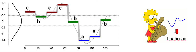
As discretization is probably the most used transformation in data mining, SAX has been widely used throughout the field. Find more information about SAX at its authors' pages: SAX overview by Jessica Lin, Eamonn Keogh's SAX page, or at the sax-vsm wiki page.
1.0 Simple time series to SAX conversion
To convert a time series of an arbitrary length to SAX we first need to define the alphabet cuts. Saxpy retrieves cuts for a Normal alphabet (we use size 3 here) via cuts_for_asize:
from saxpy.alphabet import cuts_for_asize
cuts_for_asize(3)
which yields an array (the leading -inf is the lower sentinel, so the array has alphabet_size entries):
array([ -inf, -0.4307273, 0.4307273])
To convert a time series to letters we use ts_to_string, not forgetting to z-Normalize the input first:
import numpy as np
from saxpy.znorm import znorm
from saxpy.sax import ts_to_string

ts_to_string(znorm(np.array([-2, 0, 2, 0, -1])), cuts_for_asize(3))
which produces a string:
'abcba'
2.0 SAX conversion with PAA aggregation (i.e., "chunking")
In order to reduce dimensionality further, PAA (Piecewise Aggregate Approximation) is usually applied before SAX. PAA splits the series into equally-sized segments and averages the points within each, so the example above reduces from five points to three letters:
import numpy as np
from saxpy.znorm import znorm
from saxpy.paa import paa
from saxpy.sax import ts_to_string
from saxpy.alphabet import cuts_for_asize

dat = np.array([-2, 0, 2, 0, -1])
dat_paa_3 = paa(znorm(dat), 3)

ts_to_string(dat_paa_3, cuts_for_asize(3))
and a three-letter string is produced:
'acb'
The two steps are also available as a single call, sax_by_chunking(series, paa_size, alphabet_size, znorm_threshold=0.01), which z-Normalizes, PAA-reduces, and discretizes in one shot:
from saxpy.sax import sax_by_chunking

sax_by_chunking(np.array([-2., 0, 2, 0, -1, 1, 3, 1, 0]), paa_size=3, alphabet_size=3)
# 'bbc'
3.0 SAX conversion via a sliding window
Typically, to investigate the structure of a time series -- to discover anomalous (i.e., discords) and recurrent (i.e., motifs) patterns -- we convert it to SAX via a sliding window. Saxpy implements this workflow in sax_via_window:
import numpy as np
from saxpy.sax import sax_via_window

dat = np.array([0., 0., 0., 0., 0., -0.270340178359072, -0.367828308500142,
                0.666980581124872, 1.87088147328446, 2.14548907684624,
                -0.480859313143032, -0.72911654245842, -0.490308602315934,
                -0.66152028906509, -0.221049033806403, 0.367003418871239,
                0.631073992586373, 0.0487728723414486, 0.762655178750436,
                0.78574757843331, 0.338239686422963, 0.784206454089066,
                -2.14265084073625, 2.11325193044223, 0.186018356196443,
                0., 0., 0., 0., 0., 0., 0., 0., 0., 0., 0.519132472499234,
                -2.604783141655, -0.244519550114012, -1.6570790528784,
                3.34184602886343, 2.10361226260999, 1.9796808733979,
                -0.822247322003058, 1.06850578033292, -0.678811824405992,
                0.804225748913681, 0.57363964388698, 0.437113583759113,
                0.437208643628268, 0.989892093383503, 1.76545983424176,
                0.119483882364649, -0.222311941138971, -0.74669456611669,
                -0.0663660879732063, 0., 0., 0., 0., 0.,])

sax_via_window(dat, win_size=6, paa_size=3, alphabet_size=3, nr_strategy=None, znorm_threshold=0.01)
the result maps each SAX word to the list of start positions where it occurred:
defaultdict(list,
            {'aac': [4, 10, 11, 30, 35],
             'abc': [12, 14, 36, 44],
             'acb': [5, 16, 21, 37, 43],
             'acc': [13, 52, 53, 54],
             'bac': [3, 19, 34, 45, 51],
             'bba': [31],
             'bbb': [15, 18, 20, 22, 25, 26, 27, 28, 29, 41, 42, 46],
             'bbc': [2],
             'bca': [6, 17, 32, 38, 47, 48],
             'caa': [8, 23, 24, 40],
             'cab': [9, 50],
             'cba': [7, 39, 49],
             'cbb': [33],
             'cca': [0, 1]})
sax_via_window is the hub almost everything downstream calls. Its full signature:
def sax_via_window(series, win_size, paa_size, alphabet_size=3,
                   nr_strategy='exact', znorm_threshold=0.01, sax_type='unidim')
nr_strategy is the numerosity reduction strategy ('exact', 'mindist', or None) that collapses runs of the same/near-identical consecutive word. sax_type selects the per-window strategy: 'unidim' (the default, for 1-D series) and the three multi-dimensional modes below.
3.1 Multi-dimensional SAX (SAX-ENERGY / SAX-REPEAT / SAX-INDEPENDENT)
For a multi-dimensional series (an n x d array of n timestamps over d dimensions), sax_type selects how the dimensions are combined [4]:
'independent'-- SAX-encode each dimension on its own and concatenate the per-dimension words;'energy'-- z-Normalize across dimensions and aggregate the per-dimension energy;'repeat'-- run standard SAX per dimension, then k-means-cluster the multi-dimensional words into the requested alphabet.
For example, on a 12-point, 2-dimensional series with the independent mode:
import numpy as np
from saxpy.sax import sax_via_window

mts = np.column_stack([np.sin(np.linspace(0, 3, 12)),
                       np.cos(np.linspace(0, 3, 12))])

sax_via_window(mts, win_size=6, paa_size=3, alphabet_size=3,
               nr_strategy="none", znorm_threshold=0.01, sax_type="independent")
# {'abccba': [0, 1], 'acccba': [2], 'acbcba': [3], 'ccacba': [4], 'cbacba': [5, 6]}
each six-letter word is the 3-letter word of dimension 0 followed by that of dimension 1.
Further reading on these variants: the paper that introduces them, Mohammad & Nishida, Robust learning from demonstrations using multidimensional SAX, ICCAS 2014 [4] (pp. 64-71); and an open-access walkthrough of the SAX-REPEAT construction for multivariate series in Figueirêdo, Guarieiro & Nascimento, Multivariate Real Time Series Data Using Six Unsupervised Machine Learning Algorithms, IntechOpen 2020, §2.3.
4.0 Time series discord discovery with HOT-SAX
Saxpy implements the HOT-SAX discord discovery algorithm in find_discords_hotsax:
import numpy as np
from saxpy import find_discords_hotsax, ecg0606_path

dd = np.genfromtxt(ecg0606_path(), delimiter=",")
find_discords_hotsax(dd)
which finds the anomalies as (position, nearest-neighbour distance) pairs:
[(430, np.float64(5.279080006171839)), (318, np.float64(4.175756357308695))]
The function is parameterized with the sliding window size, the number of discords desired, the PAA and alphabet sizes, and the z-Normalization threshold:
def find_discords_hotsax(series, win_size=100, num_discords=2, paa_size=3,
                         alphabet_size=3, znorm_threshold=0.01, sax_type='unidim')
For verifying discords or measuring the HOT-SAX speed-up, saxpy also ships a reference O(n²) brute-force search, find_discords_brute_force(series, win_size, num_discords=2, znorm_threshold=0.01):
from saxpy.discord import find_discords_brute_force

find_discords_brute_force(dd[100:500], 100, 2)
# [(73, 6.198555329625454), (219, 5.563692399101613)]
Both searches take an optional random_state for a reproducible search trajectory; the discords themselves are deterministic (lowest-index tie-break) regardless of the seed.
5.0 Grammar inference with RePair
Saxpy infers a RePair grammar from a space-delimited string of SAX words (or any tokens) via str_to_repair_grammar, which returns a dict mapping rule_id to a RepairRule. Rule 0 (R0) is the compressed top-level string:
from saxpy.repair import str_to_repair_grammar

g = str_to_repair_grammar("abc abc cba cba bac xxx abc abc cba cba bac")
g[0].rule_string           # 'R4 xxx R4'
g[4].expanded_rule_string  # 'abc abc cba cba bac'
RePair is lossless and the grammar is structurally equivalent across the R, Python, and Java implementations: decompressing R0 always reproduces the input, and R0 ends up with no repeated digram. RePair works by repeatedly replacing the most frequent digram with a new rule; when several digrams share the maximal frequency, which one is replaced first is an implementation detail (priority-queue / hash-table iteration order). On tie-heavy inputs this can change rule ids and rule count between saxpy, R, and Java even when the SAX input string is identical -- so treat rule_id as implementation-local, not a cross-language identifier. saxpy's SAX layer matches R/Java; grammar trees may still diverge above that.
6.0 Time series discord discovery with RRA
The Rare Rule Anomaly (RRA) algorithm builds a RePair grammar over the SAX representation, derives variable-length subsequences from the grammar rules, and searches them rarest-first. It is exposed as find_discords_rra:
import numpy as np
from saxpy import find_discords_rra, ecg0606_path

dd = np.genfromtxt(ecg0606_path(), delimiter=",")
find_discords_rra(dd, win_size=100, num_discords=2)
which returns a list of RRADiscord records (variable-length, with start/end positions and the nearest-neighbour distance):
[RRADiscord(rule_id=76, start=1722, end=1870, length=148, nn_distance=0.05577536309246554),
 RRADiscord(rule_id=35, start=430, end=531, length=101, nn_distance=0.05258209490111305)]
As noted in the reference section, nn_distance is computed between z-normalized subsequences (so RRA keys on shape, like HOT-SAX), and because the rarest-first search early-abandons it is a search-order-dependent approximation of the true nearest-neighbour distance; the discord positions are stable. The signature:
def find_discords_rra(series, win_size, paa_size=3, alphabet_size=3,
                      nr_strategy="none", znorm_threshold=0.01, num_discords=2,
                      random_state=None)
7.0 Time series classification with SAX-VSM
SAX-VSM turns each training class into a single "bag of words" of SAX patterns, weights those with TF*IDF, and classifies a new series by the class whose weight vector is closest in cosine angle [5]. Saxpy ships the building blocks (series_to_wordbag, manyseries_to_wordbag, bags_to_tfidf, cosine_distance, class_for_bag) and, on top of them, a convenience layer (load_ucr_data, train_tfidf, classify_series, classification_accuracy).
Using the Cylinder-Bell-Funnel dataset that ships in the repository:
from saxpy.saxvsm import load_ucr_data, train_tfidf, classification_accuracy

# UCR/jMotif text format: class label in column 0, series values after.
train = load_ucr_data("resources/data/cbf/CBF_TRAIN")  # {'1': [...], '2': [...], '3': [...]}
test  = load_ucr_data("resources/data/cbf/CBF_TEST")

# build the per-class TF*IDF vectors, then score the test split
tfidf = train_tfidf(train, win_size=60, paa_size=8, alphabet_size=6,
                    nr_strategy="exact", znorm_threshold=0.01)
classification_accuracy(test, tfidf, 60, 8, 6, "exact", 0.01)
# 1.0  -- a perfect score on CBF at these parameters
bags_to_tfidf takes an optional tf_scheme ("log1p", the default ln(1 + tf), or "smart", 1 + ln(tf)); see the cross-implementation note above for why log1p is canonical. To classify a single series, use classify_series(series, tfidf, win_size, paa_size, ...), which returns the predicted label (or None when every class ties).
7.1 SAX-VSM discretization parameters optimization
The window / PAA / alphabet sizes are the hidden parameters of SAX-VSM, and the right choice is not obvious. saxpy can select them automatically by minimizing the leave-out cross-validation error on the training set with the DIRECT global optimizer (scipy.optimize.direct) -- the same recipe used by the Java DiRect sampler and the jmotif-R README:
import numpy as np
from saxpy.saxvsm_optimize import optimize_parameters

X = np.array([s for series in train.values() for s in series])
y = np.array([lbl for lbl, series in train.items() for _ in series])

optimize_parameters(X, y, max_iter=10, random_state=0)
# {'window_size': 65, 'paa_size': 12, 'alphabet_size': 4,
#  'cv_error': 0.0, 'nfev': 11, 'evaluations': [...]}
optimize_parameters is deterministic for a fixed random_state; the underlying CV objective is exposed separately as cv_error(train_data, train_labels, params, ...) if you want to score a single parameter point. Run independently, saxpy, jmotif-R, and Java each pick their own optimum and reach the same test accuracy on the datasets we checked (CBF, Coffee, Gun_Point, Beef).
8.0 Time series motif discovery with EMMA
Not implemented in saxpy, and not planned. EMMA (the complement to HOT-SAX -- recurrent motifs rather than discords) is available in the sibling Java project. A Python port is out of scope for this reference package; use the Java implementation for EMMA motif discovery.
Algorithm performance
The tables below characterize the time and peak-memory behaviour of the saxpy algorithms as a function of series length. Each row is a real, non-periodic signal at that length (tiling/exact repetition makes the discord search pathological, so it is avoided), discretized with win=100, paa=4, alphabet=4, finding two discords. Measured on an AMD Ryzen 9 5950X (single core, Python 3.12) with a standalone profiling harness. Because each length is a different signal, read the columns as real-world cost at that scale, not a controlled same-signal scaling curve.
Wall-clock (seconds, best of repeated runs):
| n | dataset | SAX via window | HOT-SAX | brute-force | RePair | RRA |
|---|---|---|---|---|---|---|
| 2,299 | ecg0606 | 0.16 | 0.82 | 0.82 | 0.005 | 2.08 |
| 5,400 | stdb_308 | 0.38 | 9.36 | 4.28 | 0.009 | 18.94 |
| 21,600 | mitdbx_108 | 1.52 | 19.31 | 76.53 | 0.030 | 77.22 |
| 35,039 | dutch_power | 2.49 | 71.50 | 232.44 | 0.066 | 195.97 |
Peak memory (MiB above baseline, via tracemalloc):
| n | dataset | SAX via window | HOT-SAX | brute-force | RePair | RRA |
|---|---|---|---|---|---|---|
| 2,299 | ecg0606 | 0.1 | 3.7 | 3.9 | 0.2 | 1.2 |
| 5,400 | stdb_308 | 0.1 | 8.9 | 9.3 | 0.5 | 2.5 |
| 21,600 | mitdbx_108 | 0.3 | 35.9 | 37.8 | 1.3 | 9.6 |
| 35,039 | dutch_power | 0.6 | 58.4 | 61.8 | 2.6 | 16.4 |
A few things this makes concrete: sax_via_window and RePair are effectively linear and cheap in algorithm terms (RePair runs over the SAX word string, not the raw series). The tables below characterize saxpy as a reference Python implementation -- useful for scale, not as a substitute for R/Java when raw speed matters. Brute-force and HOT-SAX are O(n²) distance searches; RRA is grammar-driven and the heaviest step at large n in Python.
SAX-VSM (Cylinder-Bell-Funnel, 30 train / 900 test):
| operation | wall-clock | peak memory |
|---|---|---|
train_tfidf + classification_accuracy (all 900 test series) | 8.6 s | 0.5 MiB |
optimize_parameters (max_iter=10, leave-out CV) | 86.0 s | 1.8 MiB |
Changes since the last release
2.0.1 (Jul 2026) — user-facing packaging (no algorithm changes). The wheel bundles the
ecg0606 sample (from saxpy import ecg0606_path), stable top-level exports, and a
Getting started section (venv-first pip install, quick start, import cheat sheet).
Live on PyPI. See CHANGELOG.md.
python3 -m venv ~/venvs/saxpy && source ~/venvs/saxpy/bin/activate
pip install saxpy==2.0.1
2.0.0 — first modern PyPI release (the only prior artifact was the legacy 1.0.1.dev167 pbr snapshot). Highlights:
- New: SAX-VSM classification -- the classifier layer (§7.0) and a DIRECT cross-validation parameter optimizer (§7.1), verified identical to the R and Java implementations on CBF.
- New: the grammar layer -- RePair grammar inference (§5.0) and RRA variable-length discord discovery (§6.0), ported from the C++/Java.
- New: reproducibility -- an optional
random_stateon the HOT-SAX, brute-force, and RRA discord searches. - Reference Python port -- pip-installable, readable, aligned to R/Java at the SAX layer; not built as production machinery (see the reference section).
- Cross-implementation alignment -- z-Norm, PAA, discord distances, and SAX-VSM
log1pTF*IDF follow the jMotif stack; early NumPy vectorization on PAA was reverted so the lowest layer stays aligned. - Performance -- a bucketed priority queue for RePair (~2.8×), a lighter RRA z-Norm path (~3--6×) where it does not compromise reference semantics.
- Modernized packaging & tooling -- pbr → Hatchling,
uv+pyproject.toml, ruff + mypy gates, and a 3.10/3.11/3.12 × linux/macOS/windows CI matrix. The minimum Python is now 3.10. - Renamed
cosine_similarity→cosine_distance(it returns1 - cosine); the old name is kept as a deprecated alias.
References
[1] Lin, J., Keogh, E., Patel, P., and Lonardi, S., Finding Motifs in Time Series, The 2nd Workshop on Temporal Data Mining, the 8th ACM Int'l Conference on KDD (2002)
[2] Patel, P., Keogh, E., Lin, J., Lonardi, S., Mining Motifs in Massive Time Series Databases, In Proc. ICDM (2002)
[3] Keogh, E., Lin, J., Fu, A., HOT SAX: Efficiently finding the most unusual time series subsequence, In Proc. ICDM (2005)
[4] Mohammad, Y., Nishida T., Robust learning from demonstrations using multidimensional SAX, 2014 14th International Conference on Control, Automation and Systems (ICCAS 2014)
[5] Senin, P., and Malinchik, S., SAX-VSM: Interpretable Time Series Classification Using SAX and Vector Space Model, Data Mining (ICDM), 2013 IEEE 13th International Conference on, pp. 1175-1180 (2013)
[6] Salton, G., Wong, A., Yang, C., A vector space model for automatic indexing, Commun. ACM 18, 11, 613-620 (1975)
[7] Larsson, N.J., and Moffat, A., Offline dictionary-based compression, In Data Compression Conference (1999)
[8] Senin, P., Lin, J., Wang, X., Oates, T., Gandhi, S., Boedihardjo, A.P., Chen, C., Frankenstein, S., Time series anomaly discovery with grammar-based compression, In Proc. of the International Conference on Extending Database Technology, EDBT (2015)
Citing this work
For the SAX stack, discord search, and SAX-VSM classifier, cite [5] (Senin & Malinchik, ICDM 2013).
For grammar-based pattern discovery (RePair, RRA), cite the GrammarViz 3.0 paper: Senin, P., Lin, J., Wang, X., Oates, T., Gandhi, S., Boedihardjo, A.P., Chen, C., Frankenstein, S., GrammarViz 3.0: Interactive Discovery of Variable-Length Time Series Patterns, ACM Trans. Knowl. Discov. Data, February 2018.
[Click here for Citation BibTeX]
Made with Aloha!