Glacier flow model
February 28, 2023 · View on GitHub
.. image:: https://raw.githubusercontent.com/munterfi/glacier-flow-model/master/docs/source/_static/logo.svg :width: 120 px :alt: https://github.com/munterfi/glacier-flow-model :align: right
================== Glacier flow model
.. image:: https://zenodo.org/badge/96700423.svg :target: https://zenodo.org/badge/latestdoi/96700423
.. image:: https://img.shields.io/pypi/v/glacier-flow-model.svg :target: https://pypi.python.org/pypi/glacier-flow-model
.. image:: https://github.com/munterfi/glacier-flow-model/workflows/check/badge.svg :target: https://github.com/munterfi/glacier-flow-model/actions?query=workflow%3Acheck
.. image:: https://readthedocs.org/projects/glacier-flow-model/badge/?version=latest :target: https://glacier-flow-model.readthedocs.io/en/latest/ :alt: Documentation Status
.. image:: https://codecov.io/gh/munterfi/glacier-flow-model/branch/master/graph/badge.svg?token=2Kh9EboLXx :target: https://codecov.io/gh/munterfi/glacier-flow-model
Modeling glaciers on a digital elevation model (DEM) based on mass balance and a modified D8 flow algorithm applied to ice.
The modeling is based on a linear relationship between altitude and mass
balance, the so-called mass balance gradient. For alpine glaciers this gradient
is about 0.006 m/m. Continental glaciers tend to be at 0.003 and maritime
glaciers at 0.01 m/m. The alpine gradient is set by default in the model.
To model the glaciers, annual steps are calculated. First the mass balance
(accumulation and ablation) for the area is added to the glacier layer and in a
second step the glacier flow is simulated by using a modified D8 technique
(submodule :code:fracd8).
Since the prupose of the D8 flow direction algorithm is modeling surface water
flows over terrain, the D8 algorithm was modified to be able to consider the
fraction of ice that is flowing out of each cell based on the glaciers
velocity. In order to avoid pure convergence of the flow, the surface of the
glaciers is slightly smoothed. The simulation stops when the observed
difference in mass balance for a smoothed curve (default
:code:MODEL_TREND_SIZE=100) is less than a given tolerance (default
:code:MODEL_TOLERANCE=0.0001).
Getting started
The glacier-flow-model package depends on GDAL, which needs to be installed on the system.
Get the stable release of the package from pypi:
.. code-block:: shell
pip install glacier-flow-model
Example data
The package includes an example DEM from swisstopo <https://www.swisstopo.admin.ch/en/home.html>_.
It covers a smaller extent around the Aletsch glacial arena in Switzerland with
a raster cell resolution of 200m.
.. code-block:: python
from glacier_flow_model import PkgDataAccess
dem = PkgDataAccess.load_dem()
The original DEM can be downloaded here <https://www.swisstopo.admin.ch/en/geodata/height/dhm25200.html>_.
Usage
To set up a glacier flow model, a path to a DEM in the GeoTiff file format has to passed to the model class constructor. By default the mass balance parameters for alpine glaciers in the year 2000 are set. Keep the input file size small, otherwise the model may be slowed down remarkably:
.. code-block:: python
import logging
from glacier_flow_model import GlacierFlowModel, PkgDataAccess

LOG_FORMAT = "[%(asctime)s %(levelname)s] %(message)s (%(name)s)"
logging.basicConfig(format=LOG_FORMAT, level=logging.INFO)

gfm = GlacierFlowModel(PkgDataAccess.locate_dem())
After initialization, the model needs to accumulate the initial ice mass until
it reaches a steady state, call the :code:reach_steady_state method to do so:
.. code-block:: python
gfm.reach_steady_state()
.. image:: https://raw.githubusercontent.com/munterfi/glacier-flow-model/master/docs/source/_static/steady_state_initial.png :alt: https://github.com/munterfi/glacier-flow-model :align: center
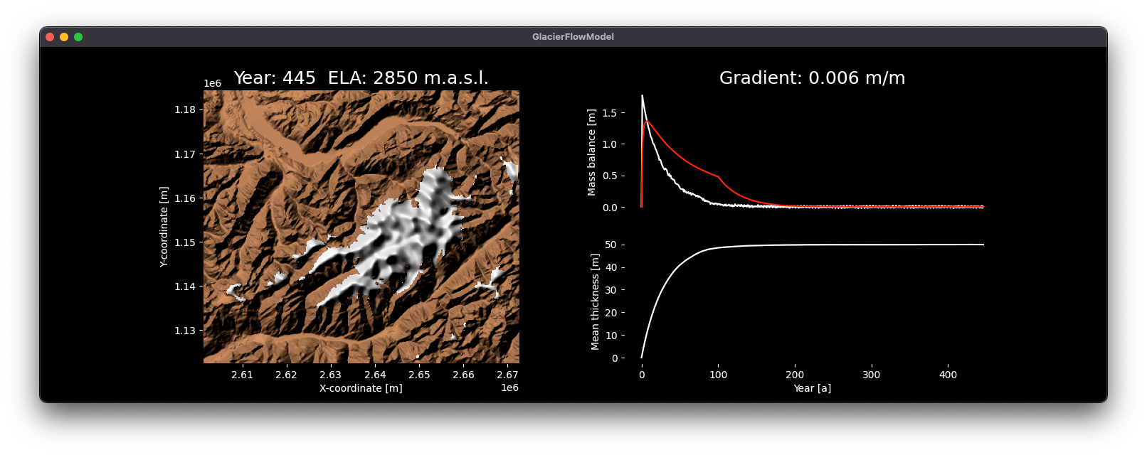
When the model is in a steady state, a temperature change of the climate can be
simulated. Simply use the :code:simulate method with a positive or negative
temperature change in degrees. The model changes the temperature gradually and
simulates years until it reaches a steady state again.
Heating 4.5°C after initial steady state:
.. code-block:: python
gfm.simulate(4.5)
.. image:: https://raw.githubusercontent.com/munterfi/glacier-flow-model/master/docs/source/_static/steady_state_heating.png :alt: https://github.com/munterfi/glacier-flow-model :align: center
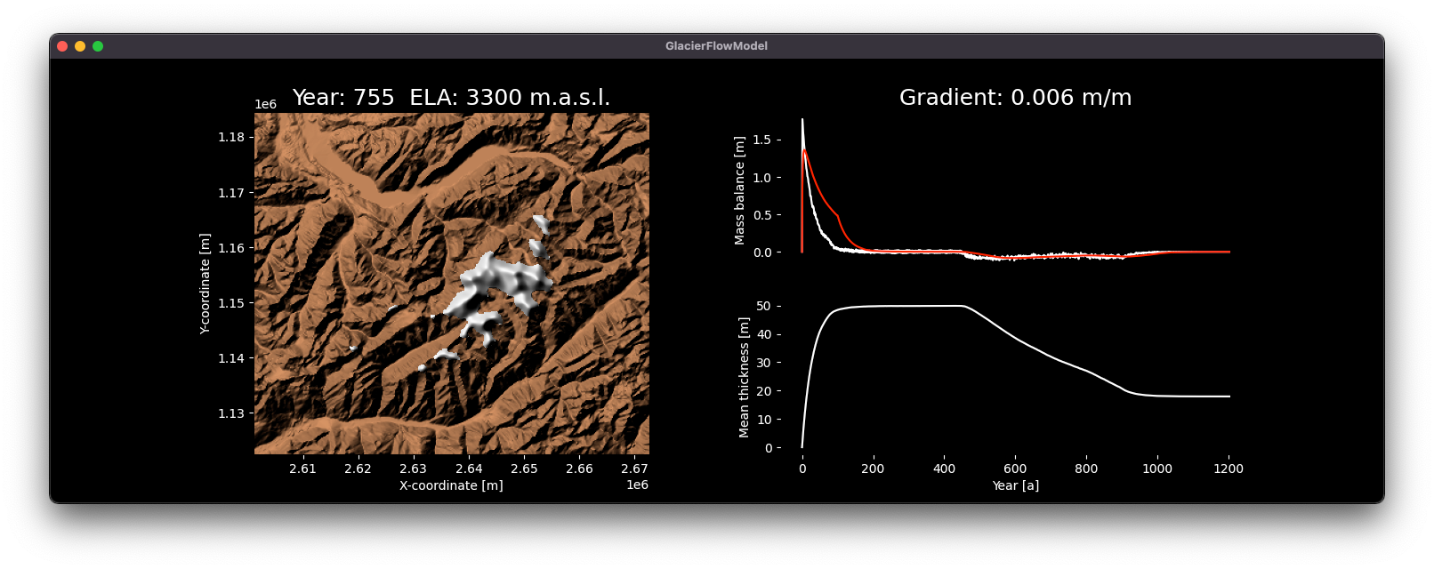
Cooling -3°C after initial steady state:
.. code-block:: python
gfm.simulate(-3)
.. image:: https://raw.githubusercontent.com/munterfi/glacier-flow-model/master/docs/source/_static/steady_state_cooling.png :alt: https://github.com/munterfi/glacier-flow-model :align: center
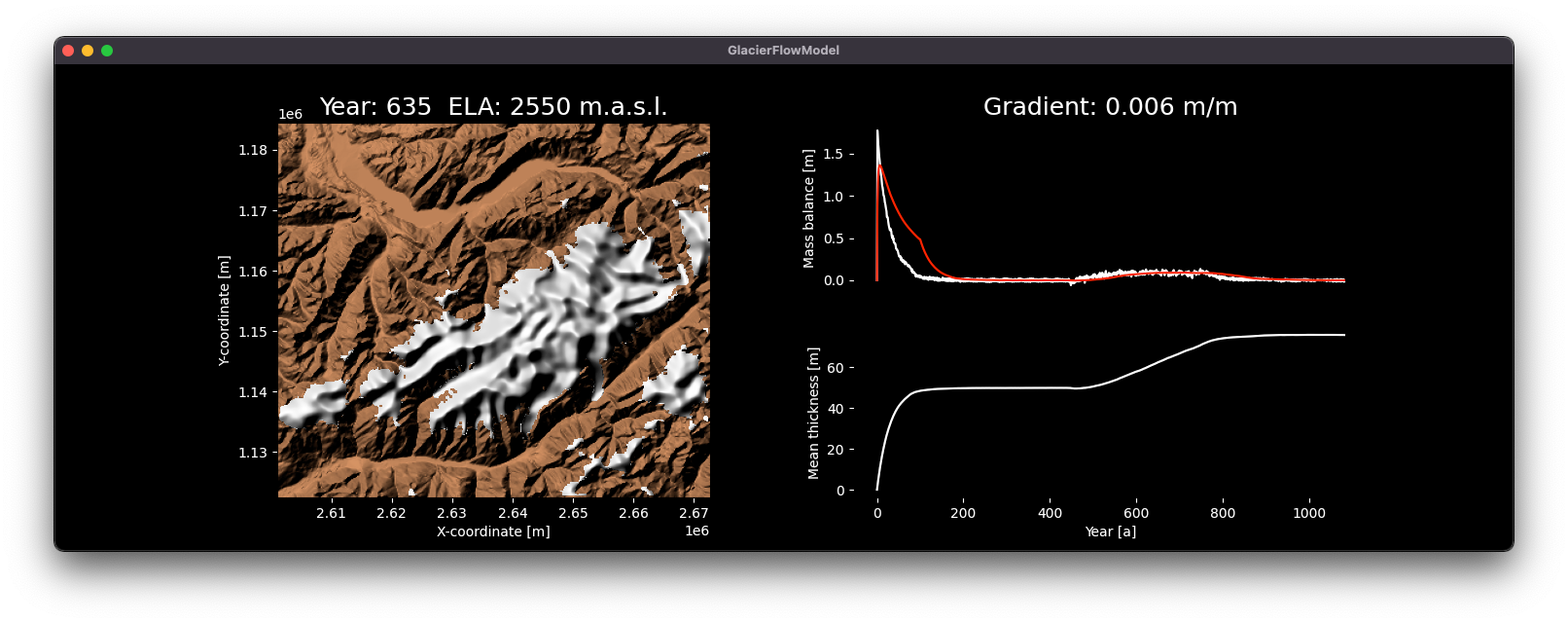
Export the results of the model into :code:.csv and :code:.tif files:
.. code-block:: python
gfm.export()
The GeoTiff contains the following bands, averaged over the last 10 simulation
years (default :code:MODEL_RECORD_SIZE=10):
- Glacier thickness [m].
- Velocity at medium height [m/a].
- Mass balance [m].
Check out the video <https://munterfinger.ch/media/film/gfm.mp4>_ of the scenario simulation in the Aletsch
glacial arena in Switzerland
Limitations
The model has some limitations that need to be considered:
- The flow velocity of the ice per year is limited by the resolution of the grid cells. Therefore, a too high resolution should not be chosen for the simulation.
- The modeling of ice flow is done with D8, a technique for modeling surface flow in hydrology. Water behaves fundamentally different from ice, which is neglected by the model (e.g. influence of crevasses).
- The flow velocity only considers internal ice deformation (creep). Basal sliding, and soft bed deformation are ignored.
- No distinction is made between snow and ice. The density of the snow or ice mass is also neglected in the vertical column.
License
This project is licensed under the MIT License - see the LICENSE file for details