Controllable 3D Outdoor Scene Generation via Scene Graphs

July 13, 2026 · View on GitHub

Controllable 3D Outdoor Scene Generation via Scene Graphs

[ICCV 2025] Yuheng Liu^1,2, Xinke Li³, Yuning Zhang⁴, Lu Qi⁵, Xin Li¹, Wenping Wang¹, Chongshou Li⁴, Xueting Li^6*, Ming-Hsuan Yang^2*

¹Texas A&M University, ²The University of Cailfornia, Merced, ³City University of HongKong, ⁴Southwest Jiaotong University, ⁵Insta360 Research, ⁶NVIDIA

Teaser

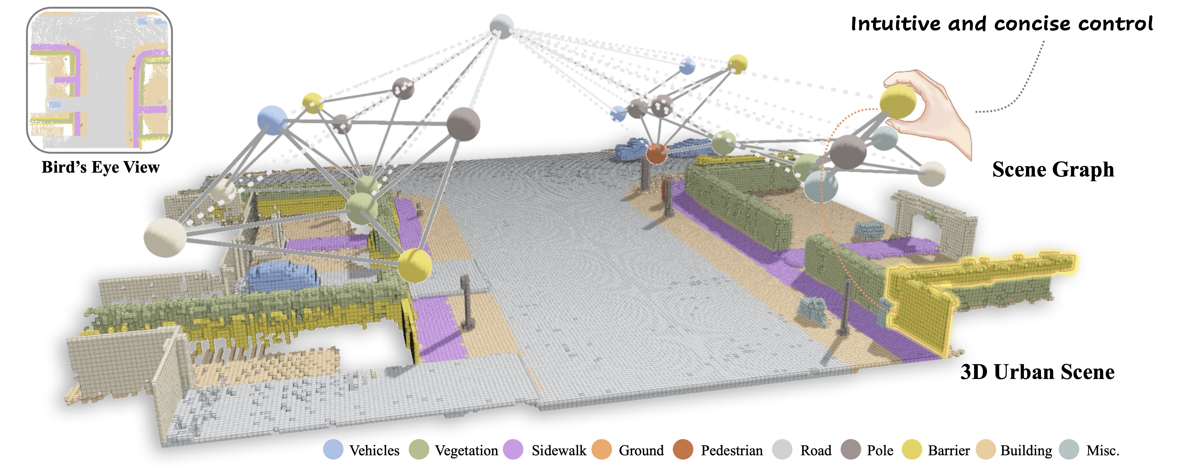
Three-dimensional scene generation is crucial in computer vision, with applications spanning autonomous driving, gaming and the metaverse. Current methods either lack user control or rely on imprecise, non-intuitive conditions. In this work, we propose a method that uses scene graphs—an accessible, user-friendly control format—to generate outdoor 3D scenes. We develop an interactive system that transforms a sparse scene graph into a dense BEV (Bird's Eye View) Embedding Layout, which guides a conditional diffusion model to generate 3D scenes that match the scene graph description. During inference, users can easily create or modify scene graphs to generate large-scale outdoor scenes. We create a large-scale dataset with paired scene graphs and 3D semantic scenes to train the BEV embedding and diffusion models. Experimental results show that our approach consistently produces high-quality 3D urban scenes closely aligned with the input scene graphs.

NEWS

[2026/07/13] Training and inference code is released.
[2025/06/25] Our work is accepted by ICCV 2025.
[2025/03/10] Our work is now on arXiv.
[2024/11/15] Official repo is created, code will be released soon.

Overview

Given a sparse scene graph, our method first converts it into a dense BEV Embedding Map (BEM), generates a 2D bird's-eye-view semantic map with a discrete diffusion model, and then lifts that map into a first-stage 3D semantic scene with a second, conditional discrete diffusion model. The coarse 3D scene is further up-scaled to high resolution with our sister project, Pyramid Discrete Diffusion (PDD).

Installation
Data Preparation
Training
Inference
Multi-GPU
Repository Layout
Configuration Reference
Citation

Installation

conda create -n control-3d-scene python=3.10 -y
conda activate control-3d-scene

# 1) Install PyTorch matching your CUDA (example: CUDA 11.8)
pip install torch --index-url https://download.pytorch.org/whl/cu118

# 2) torch_scatter must match your torch/CUDA build
pip install torch_scatter -f https://data.pyg.org/whl/torch-2.7.1+cu118.html

# 3) The rest
pip install -r requirements.txt

Verify:

python -c "import torch, torch_geometric, torch_scatter, einops, numba; print('ok', torch.cuda.is_available())"

Data Preparation

Two ingredients are needed: the scene graphs (provided) and the CarlaSC voxel scenes (downloaded and processed here).

1. Scene graphs (CarlaSG)

The paired scene-graph annotations are released as CSV files (carla_scene_graph_v5). Place them under data/:

data/carla_scene_graph_v5/
├── train/{nodes.csv, edges.csv}
├── val/{nodes.csv, edges.csv}
└── test/{nodes.csv, edges.csv}

Each nodes.csv row is file_path, instance_id, label_id, position, road_type, centroid; each edges.csv row is file_path, subject_instance_id, object_instance_id. The file_path links a scene graph to its CarlaSC frame.

2. CarlaSC voxels

Download the CarlaSC Finer split (same data used by PDD) and extract it into data/:

# ~4.4 GB download, ~90 GB extracted
wget https://curly-dataset-public.s3.us-east-2.amazonaws.com/CARLA/eval_fine.zip -P data/
unzip -q data/eval_fine.zip -d data/
# -> data/Cartesian/{Train,Val,Test}/Town##_*/cartesian/evaluation_fine/*.label

Then process the raw 256×256×16 voxels into the 64×64×8 scenes and 64×64 BEV maps used for training:

python tools/prepare_carla.py \
    --carla_root data/Cartesian \
    --out_root   data/CarlaSG \
    --splits Train Val Test \
    --workers 16

This writes, mirroring each scene-graph file_path:

data/CarlaSG/scene/<split>/Town.../evaluation_fine/*.npy   # 64×64×8 3D scene (stage-2 target)
data/CarlaSG/bev/<split>/Town.../evaluation_fine/*.npy     # 64×64 BEV map  (stage-1 target / stage-2 condition)

The 23 raw CarlaSC classes are remapped to 11 classes (see datasets/carla.yaml), the 3D scene is a majority-vote down-sampling, and the BEV map is a priority-based top-down projection that keeps sparse foreground objects (vehicles, pedestrians, poles) visible so they remain controllable.

You can process a subset first with --limit 200 to smoke-test the pipeline.

Training

Training follows the paper's best strategy: jointly train the GNN and the 2D diffusion model (with ground-truth positions), then post-train the localization head, and separately train the 3D diffusion model.

Stage 1 — joint GNN + 2D map diffusion

python launch.py -c configs/train_sg_to_bev.yaml -n sg_to_bev

Stage 1 — localization-head post-training (loads the checkpoint above)

python launch.py -c configs/posttrain_loc.yaml -n posttrain_loc \
    --resume_path ./checkpoints/sg_to_bev/latest.tar

Stage 2 — 2D map → 3D scene diffusion

python launch.py -c configs/train_bev_to_3d.yaml -n bev_to_3d

Checkpoints are written to ./checkpoints/<exp_name>/. Any config field can be overridden on the command line, e.g. --batch_size 8 --lr 0.002 --epochs 500.

Inference

Stage 1 — scene graph → BEV map

python launch.py -c configs/infer_sg_to_bev.yaml -n infer_sg_to_bev \
    --resume_path ./checkpoints/posttrain_loc/latest.tar
# -> ./generated/infer_sg_to_bev/Generated/*.npy   (+ .ply under GeneratedPly/)

Stage 2 — BEV map → 3D scene (end-to-end, consuming stage-1 output)

python launch.py -c configs/infer_bev_to_3d.yaml -n infer_bev_to_3d \
    --resume_path ./checkpoints/bev_to_3d/latest.tar \
    --infer_source generation \
    --prev_scene_path ./generated/infer_sg_to_bev/Generated
# -> ./generated/infer_bev_to_3d/Generated/*.npy   (64×64×8 scenes, + .ply)

Set --infer_source dataset to instead condition stage 2 on ground-truth BEV maps (useful for sanity checking stage 2 in isolation).

High-resolution up-scaling. Feed the generated 64×64×8 scenes to PDD (its S_2 → S_3 stage) to obtain 256×256×16 scenes. The .npy label format is compatible with PDD's visualizer.

.ply point clouds are written alongside the .npy outputs and open directly in MeshLab / CloudCompare / Open3D.

Multi-GPU

List the GPUs to use under gpus in the config and set distribution: true (training only; inference uses a single GPU). No torchrun needed — the launcher spawns one process per GPU and wraps the model in DistributedDataParallel:

# train stage 1 on GPUs 6 and 7
python launch.py -c configs/train_sg_to_bev.yaml -n sg_to_bev \
    --gpus 6 7 --distribution true

Repository Layout

configs/                 YAML configs for each stage / mode
datasets/
  carla.yaml             class remapping, colors, frequencies
  scene_graph_dataset.py CarlaSG dataset (scene graph + BEV + 3D)
  data.py                dataloader construction (train / inference, DDP sampler)
models/
  gnn.py                 GAT encoder, CANE, edge-recon & node-cls heads, localization head
  allocation.py          BEM assembly, Gumbel position sampling, overlap resolution
  diffusion.py           conditional discrete (multinomial) diffusion
  denoise.py             3D-UNet denoiser (shared by both stages)
  sg_to_bev.py           Stage 1 model (scene graph → 2D map)
  bev_to_3d.py           Stage 2 model (2D map → 3D scene)
tools/
  prepare_carla.py       CarlaSC voxels → 64×64×8 scenes + 64×64 BEV maps
utils/                   config, distributed launch, optimizer, visualization
launch.py                entry point (train / loc_posttrain / inference)
train.py                 training loop
generate.py              inference loop

Configuration Reference

Key	Meaning
`stage`	`sg_to_bev` (stage 1) or `bev_to_3d` (stage 2)
`mode`	`train`, `loc_posttrain`, or `inference`
`gnn_hidden`	GAT hidden / CANE dimension `C` (default 32)
`diffusion_steps`	number of discrete diffusion steps (default 100)
`recon_loss_weight`, `seg_loss_weight`	weights of the edge-reconstruction and node-classification auxiliary tasks
`uncond_prob`	fraction of samples trained with an all-ones (unconditional) BEM
`feature_mask_ratio`	probability of dropping a node's position feature during stage-1 training
`gumbel_tau`	temperature for position sampling at inference (higher → more diverse)
`overlap_move`	pixels by which colliding node positions are nudged apart
`gpus`, `distribution`	GPU ids and multi-GPU toggle
`infer_source`	stage-2 inference condition: `dataset` (GT BEV) or `generation` (stage-1 output)
`prev_scene_path`	directory of stage-1 BEV maps when `infer_source=generation`

Citation

If you find our work useful, please cite:

@inproceedings{liu2025controllable,
  title     = {Controllable 3D Outdoor Scene Generation via Scene Graphs},
  author    = {Liu, Yuheng and Li, Xinke and Zhang, Yuning and Qi, Lu and Li, Xin
               and Wang, Wenping and Li, Chongshou and Li, Xueting and Yang, Ming-Hsuan},
  booktitle = {ICCV},
  year      = {2025}
}

@inproceedings{liu2024pyramid,
  title     = {Pyramid Diffusion for Fine 3D Large Scene Generation},
  author    = {Liu, Yuheng and Li, Xinke and Li, Xueting and Qi, Lu and Li, Chongshou and Yang, Ming-Hsuan},
  booktitle = {ECCV},
  year      = {2024}
}

Acknowledgements

This project builds on Pyramid Discrete Diffusion and uses the CarlaSC dataset.

License

Released under the MIT License.